BAS files here
unsigned notes page here GI CRC template here OORAM page here
Basics:
Filter by a particular value in a cell & copy the entire row to another worksheet: view code here
Best Achievements:
Unsigned Orders Template 5.26.22 video works with Unsigned Orders Template 5.26.22 excel macro file
Templates:
Use Userform to Enter Data - NL 4.22.22
Books:
Excel VBA Programming Brilliant (Frye):
cc3 Data & Variables | cc4 Workbooks files | cc5 worksheets | cc6 Ranges | cc7 Cells | cc8 Format Worksheets Elements | cc9 Sort & Filter Data |
Excel 2016 Power Programming with VBA (Alexander):
cc2 Intro VBA | cc3-vba Prgm Fundamentals | cc4-vbaSubprocedures.pdf | cc5: function Procedures | cc6 Excel Events | cc7-Program Examples | xxxxx |
Excel Macros for Dummies 2015:
cc1 macroFundamentals | cc2-vba Editor | cc3-macros | cc4-wkbks | cc5-wkshts | cc6-range | cc7-manipData | cc8-automateTasks |cc9_emails_excel |cc10-vbeTips | cc11-macroHelp | cc12-speedUpMacros |
Videos:
How to match columns between 2 tabs NL -- 5 stars
howTo_filterIntoTabs_1.16.21a NL -- 5 stars
Filter into tabs, create tabs via array, autofit, trim cell values 2.23.21 -- NL 5 stars!
How to Build Covid-19 tracker in Excel using VBA --NL 6 stars!
5 Killer Excel VBA Tips Everyone Should Know -- Excel Macro Mastery
OORAM - how to- part 1 ---> OORAM - how to - part 2
OORAM_VBA - explaining ROWSOURCE
https://www.youtube.com/watch?v=QGFANQ4lPMA - 7 Simple Practices for Writing Super-Readable VBA Code
How to autofit columns in entire workbook --NL 2.23.21 5-stars!
How to take a spreadsheet, find uniques, put double quotes around uniques to create array, then loop array to create tabs and filter where column values = array values NL 4.22.21 a --on YouTube
How to Create Custom Word Docs From Excel w/o mail merge (form letters)
Manipulate VistA Unsigned Notes file using VBA --NL 5.18.21
Create tabs, Filter, Use arrays for Unsigned Orders DoD -- NL 5.28.21 on YoutubeNL
Files:
Code for Building COVID-19 Excel tracker --webpage from NL
VBA Code for AHLTA last sign ons
Shift-tab
Ctrl-space --> brings up intellisense to help give you options
You can interrupt a macro in Excel at any time by pressing Esc or Ctrl + Break.
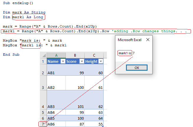
Find the last non-blank cell in a single row or column
Sub Range_End_Method()
'Finds the last non-blank cell in a single row or column

Dim lRow As Long
Dim lCol As Long

    'Find the last non-blank cell in column A(1)
    lRow = Cells(Rows.Count, 1).End(xlUp).Row

    'Find the last non-blank cell in row 1
    lCol = Cells(1, Columns.Count).End(xlToLeft).Column

    MsgBox "Last Row: " & lRow & vbNewLine & _
            "Last Column: " & lCol

End Sub
Range("C" & processRowBegin & ":C" & processRowEnd)
The below code copy Sheet1 A1 to Sheet2 B1.
Sheets("Sheet1").Range("A1").Copy (Sheets("Sheet2").Range("B1"))
Resize(1, rg.Columns.Count).Value is used to obtain the values of the specified range (rg) but limited to 1 row & the same number of columns as the original range. .Value is a property of the Range object that represents the value of the cells in the range.
shOutput.Range("A" & row).Resize(1, rg.Columns.Count).Value = rg.Rows(i).Value
shOutput: This is a Worksheet object representing a worksheet in the workbook.
Range("A" & row): This part refers to a specific cell in column A of the shOutput worksheet. The & is used for concatenation, and row is a variable representing the row number.
.Resize(1, rg.Columns.Count): This part resizes the range to cover 1 row and the same number of columns as the original range (rg). This ensures that the entire row is copied.
.Value: This sets the value of the target range (in shOutput) equal to the value of the corresponding row in the source range (rg).
= rg.Rows(i).Value: This part specifies the source range (rg) and the specific row (i) to copy. rg.Rows(i) refers to the entire ith row in the source range.
Best Videos
Copy Data to another Excel workbook based on sales and date criteria using VBA Dinesh
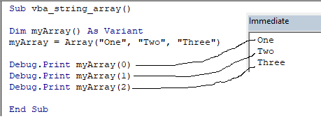
Sub vba_string_array()
Dim myArray() As Variant
myArray = Array("One", "Two", "Three")
Debug.Print myArray(0)
Debug.Print myArray(1)
Debug.Print myArray(2)
End Sub
Double Each element's value contained in an Array
Sub vba_array_loop()
Dim myArray(5) As Integer
myArray(1) = 10
myArray(2) = 20
myArray(3) = 30
myArray(4) = 40
myArray(5) = 50
Dim uB As Integer, lB As Integer
uB = UBound(myArray)
LB = LBound(myArray)
For i = LB To uB
myArray(i) = myArray(i) * 2
Next i
Debug.Print myArray(5)
End Sub
Source: https://excelchamps.com/vba/arrays/vba-loop-array/#More_on_VBA_Arrays
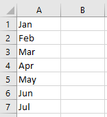
Use array to populate a column in Excel
Sub Array_Size()
Dim MyArray As Variant
MyArray = Array("Jan", "Feb", "Mar", "Apr", "May", "Jun", "Jul")
Dim k As Integer
For k = 0 To 6
Cells(k + 1, 1).Value = MyArray(k)
Next k
End Sub
Video: capitalize top cells of each column NL 4.2.22
Video:
Convert column into comma separated list in Excel Ctrl-H, ^p --> replace with ','
How to autofit columns in entire workbook --NL 2.23.21 5-stars!
Sub AutoFitAllWorksheets()
Dim ws As Worksheet
' Loop through each worksheet in the workbook
For Each ws In ThisWorkbook.Worksheets
' Autofit all columns in the current worksheet
ws.Columns.AutoFit
Next ws
End Sub
Videos:
How to make your Excel VBA code run 1000 times faster. -- Excel Macro Mastery
Set Cell value
This will set the range A2’s value = 1:
Range("A2").Value = 1
Instead of referencing a single cell, you can reference a range of cells and change all of the cell values at once:
Range("A2:A5").Value = 1
In the above examples, we set the cell value equal to a number (1). Instead, you can set the cell value equal to a string of text. In VBA, all text must be surrounded by quotations:
Range("A2").Value = "Text"
If you don’t surround the text with quotations, VBA will think you referencing a variable…
You can also set a cell value equal to a variable
Dim strText as String
strText = "String of Text"

Range("A2").Value = strText
To get the ActiveCell value and display it in a message box:
MsgBox ActiveCell.Value
To get a cell value and assign it to a variable:
Dim var as Variant

var = Range("A1").Value
Here we used a variable of type Variant. Variant variables can accept any type of values. Instead, you could use a String variable type:
Dim var as String

var = Range("A1").Value
A String variable type will accept numerical values, but it will store the numbers as text.
If you know your cell value will be numerical, you could use a Double variable type (Double variables can store decimal values):
Dim var as Double

var = Range("A1").Value
However, if you attempt to store a cell value containing text in a double variable, you will receive an error.
It’s easy to set a cell value equal to another cell value (or “Copy” a cell value):
Range("A1").Value = Range("B1").Value
You can even do this with ranges of cells (the ranges must be the same size):
Range("A1:A5").Value = Range("B1:B5").Value
You can compare cell values using the standard comparison operators.
Test if cell values are equal:
MsgBox Range("A1").Value = Range("B1").Value
Will return TRUE if cell values are equal. Otherwise FALSE.
You can also create an If Statement to compare cell values:
If Range("A1").Value > Range("B1").Value Then

  Range("C1").Value = "Greater Than"

Elseif Range("A1").Value = Range("B1").Value Then

  Range("C1").Value = "Equal"

Else

  Range("C1").Value = "Less Than"

End If
You can compare text in the same way
Source: https://www.automateexcel.com/vba/cell-value-get-set/
As you have seen you can only access one cell using the Cells property. If you want to return a range of cells then you can use Cells with Ranges as follows
' https://excelmacromastery.com/
Public Sub UsingCellsWithRange()

    With Sheet1
        ' Write 5 to Range A1:A10 using Cells property
        .Range(.Cells(1, 1), .Cells(10, 1)).Value2 = 5

        ' Format Range B1:Z1 to be bold
        .Range(.Cells(1, 2), .Cells(1, 26)).Font.Bold = True

    End With

End Sub
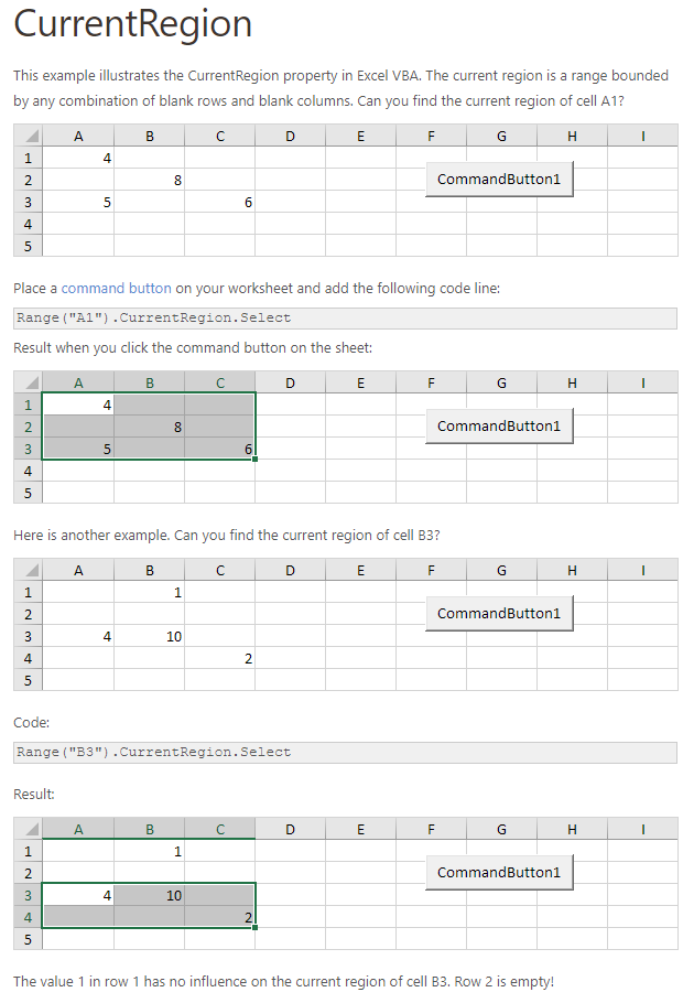
CurrentRegion returns a range of all the adjacent cells to the given range.
In the screenshot below you can see the two current regions. I have added borders to make the current regions clear.
A row or column of blank cells signifies the end of a current region.
You can manually check the CurrentRegion in Excel by selecting a cell or cells & pressing Ctrl + Shift + *.
If we take any range of cells within the border and apply CurrentRegion, we will get back the range of cells in the entire area.
For example
Range(“B3”).CurrentRegion will return the range B3:D14
Range(“D14”).CurrentRegion will return the range B3:D14
Range(“C8:C9”).CurrentRegion will return the range B3:D14
and so on
Remove header row(i.e. first row) from the range. For example if range is A1:D4 this will return A2:D4
' Current region will return B3:D14 from above example
Dim rg As Range
Set rg = Sheet1.Range("B3").CurrentRegion

' Remove Header
Set rg = rg.Resize(rg.Rows.Count - 1).Offset(1)

' Start at row 1 as no header row
Dim i As Long
For i = 1 To rg.Rows.Count
    ' current row, column 1 of range
    Debug.Print rg.Cells(i, 1).Value2
Next i
Source: https://excelmacromastery.com/excel-vba-range-cells/
Use the .Clear method.
Sheets("Test").Range("A1:C3").Clear
![]()
![]()
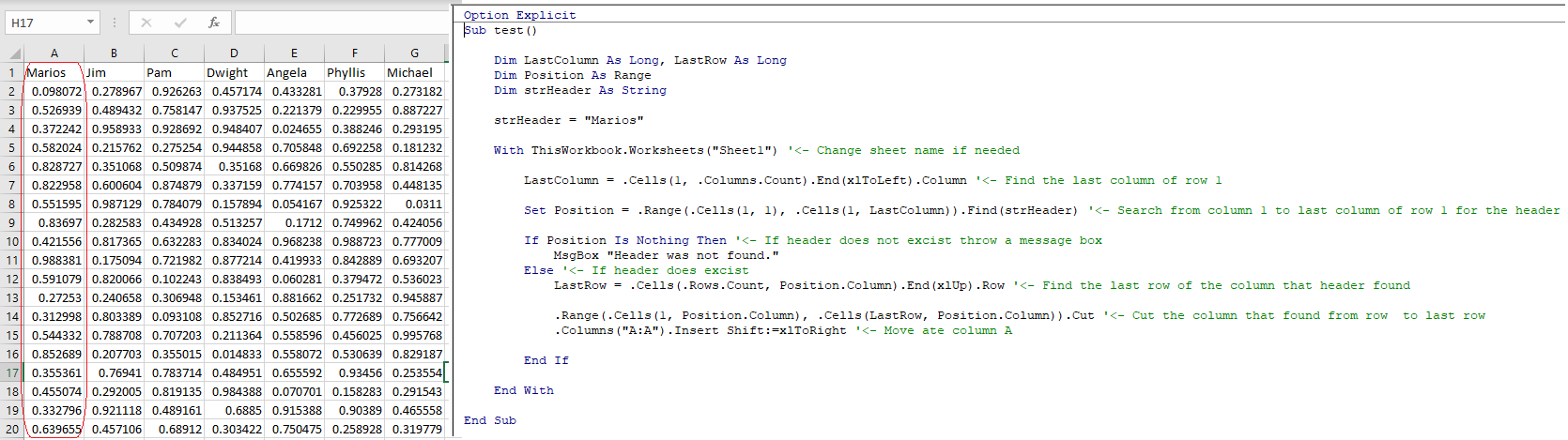
Sub test()
Dim LastColumn As Long, LastRow As Long
Dim Position As Range
Dim strHeader As String
strHeader = "Marios"
With ThisWorkbook.Worksheets("Sheet1") '<- Change sheet name if needed
LastColumn = .Cells(1, .Columns.Count).End(xlToLeft).Column '<- Find the last column of row 1
Set Position = .Range(.Cells(1, 1), .Cells(1, LastColumn)).Find(strHeader) '<- Search from column 1 to last column of row 1 for the header
If Position Is Nothing Then '<- If header does not excist throw a message box
MsgBox "Header was not found."
Else '<- If header does excist
LastRow = .Cells(.Rows.Count, Position.Column).End(xlUp).Row '<- Find the last row of the column that header found
.Range(.Cells(1, Position.Column), .Cells(LastRow, Position.Column)).Cut '<- Cut the column that found from row to last row
.Columns("A:A").Insert Shift:=xlToRight '<- Move ate column A
End If
End With
End Sub
Source: https://stackoverflow.com/questions/55701230/find-column-header-by-name-and-move-all-data-below-column-header-excel-vba/55701752
Sub Count_Rows_Example1()
Dim No_Of_Rows As Integer
No_Of_Rows = Range("A1:A8").Rows.Count
MsgBox No_Of_Rows
End Sub
or. . .
Sub Count_Rows_Example2()

Dim No_Of_Rows As Integer

No_Of_Rows = Range("A1").End(xlDown).Row

MsgBox No_Of_Rows

End Sub
or. . .
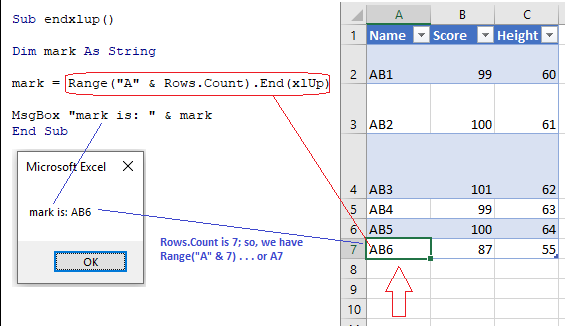
Sub Count_Rows_Example3()

Dim No_Of_Rows As Integer

No_Of_Rows = Cells(Rows.Count, 1).End(xlUp).Row

MsgBox No_Of_Rows

End Sub
Source: https://www.wallstreetmojo.com/vba-row-count/
or. . .
Sub Test()
    With ActiveSheet
    lastRow = .Cells(.Rows.Count, "A").End(xlUp).Row
    MsgBox lastRow
    End With
End Sub
Private Sub CommandButton2_Click()

Dim A As Integer
Dim Count As Integer
Dim LRow As Long

LRow = Range("A1").CurrentRegion.End(xlDown).Row

For A = 1 To LRow

If Cells(A, 1).Value > 10 Then
Count = Count + 1
Cells(A, 1).Font.ColorIndex = 44  'Gold
Else
Cells(A, 1).Font.ColorIndex = 55  'Blue
End If

Next A

Cells(2, 4).Value = Count
Cells(3, 4).Value = 12 - Count

End Sub
Source: https://www.educba.com/vba-counter/ 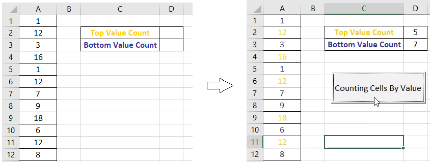
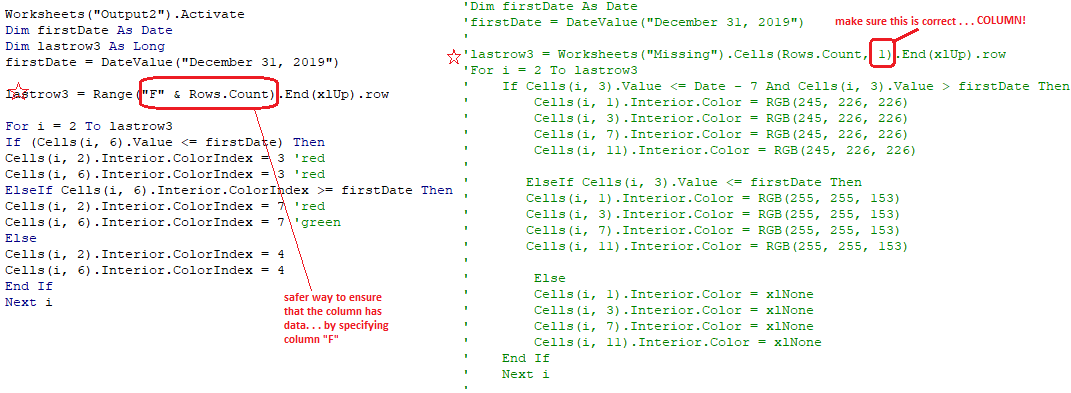
Worksheets("Output2").Activate
Dim firstDate As Date
Dim lastrow3 As Long
lastrow3 = Worksheets("Output2").Cells(Rows.Count, 6).End(xlUp).row 'specify correct column, please
firstDate = DateValue("December 31, 2019")
For i = 2 To lastrow3
If Cells(i, 6).Value <= Date - 7 And Cells(i, 6).Value > firstDate Then ' "Date - 7" means a week ago from today's date
Cells(i, 1).Interior.Color = RGB(245, 226, 226)
Cells(i, 6).Interior.Color = RGB(245, 226, 226)
Cells(i, 7).Interior.Color = RGB(245, 226, 226)
Cells(i, 11).Interior.Color = RGB(245, 226, 226)
ElseIf Cells(i, 3).Value <= firstDate Then
Cells(i, 1).Interior.Color = RGB(255, 255, 153)
Cells(i, 6).Interior.Color = RGB(255, 255, 153)
Cells(i, 7).Interior.Color = RGB(255, 255, 153)
Cells(i, 11).Interior.Color = RGB(255, 255, 153)
Else
Cells(i, 1).Interior.Color = xlNone
Cells(i, 6).Interior.Color = xlNone
Cells(i, 7).Interior.Color = xlNone
Cells(i, 11).Interior.Color = xlNone
End If
Next i
Or. . .
Worksheets("Output2").Activate
Dim firstDate As Date
Dim lastrow3 As Long
firstDate = DateValue("December 31, 2019")
lastrow3 = Range("F" & Rows.Count).End(xlUp).row ' "F" is column F
For i = 2 To lastrow3
If (Cells(i, 6).Value <= Date - 7) Then
Cells(i, 2).Interior.ColorIndex = 3 'red
Cells(i, 6).Interior.ColorIndex = 3 'red
ElseIf Cells(i, 6).Interior.ColorIndex >= Date - 7 Then
Cells(i, 2).Interior.ColorIndex = 7 'red
Cells(i, 6).Interior.ColorIndex = 7 'green
Else
Cells(i, 2).Interior.ColorIndex = 4
Cells(i, 6).Interior.ColorIndex = 4
End If
Next i
Source: https://www.youtube.com/watch?v=lgec4z5hajs
Sub ConslidateWorkbooks()
Dim FolderPath As String
Dim FileName As String
Dim Sheet As Worksheet
Application.ScreenUpdating = False
FolderPath = Environ("USERPROFILE") & "\Desktop\Test\" 'Create a folder in Desktop folder named 'Test'
FileName = Dir(FolderPath & "*.xlsx*") 'make sure your files' extensions matches the code; here, my files have extension '.xlsx'
'MsgBox "Filename is " & FileName
Do While FileName <> ""
Workbooks.Open FileName:=FolderPath & FileName, ReadOnly:=True
For Each Sheet In ActiveWorkbook.Sheets
Sheet.Copy After:=ThisWorkbook.Sheets(1) 'make sure the tabs within each Excel file have the correct tab names you want to see in the new combined Excel file
Next Sheet
Workbooks(FileName).Close
FileName = Dir()
Loop
Application.ScreenUpdating = True
End Sub
Source: https://trumpexcel.com/combine-multiple-workbooks-one-excel-workbooks/
Source:
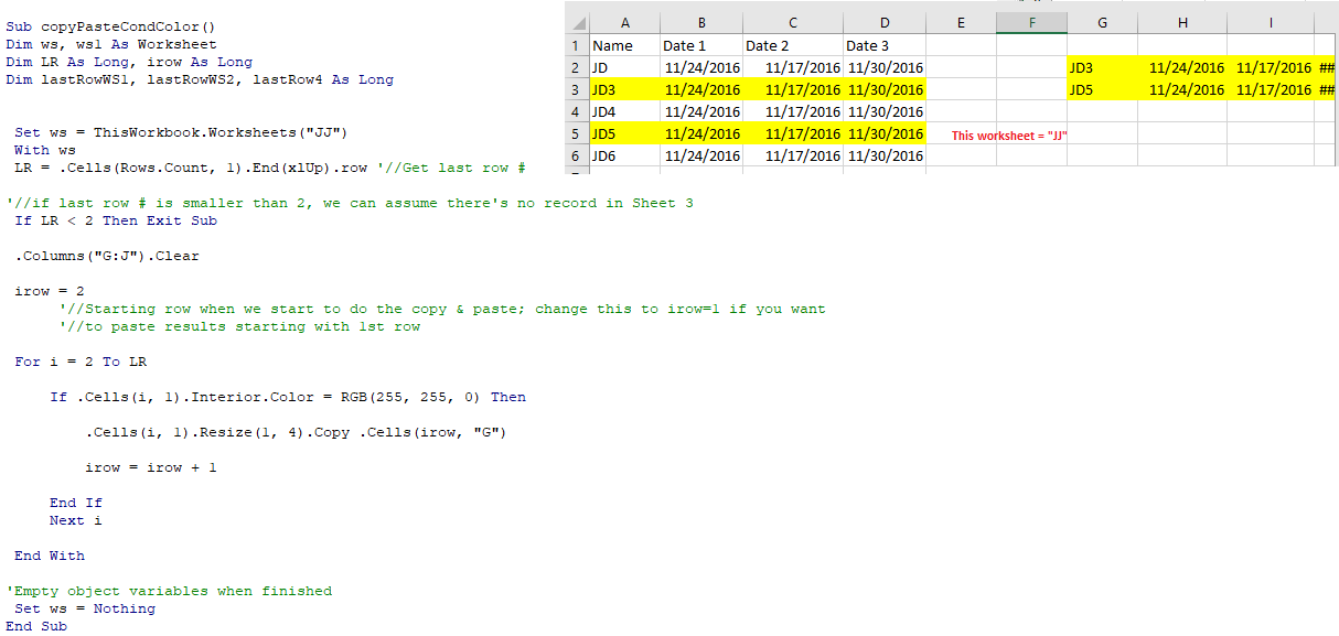
my video: here
https://www.youtube.com/watch?v=39WCiRK4iwo Copy and Paste Colored Cells To Destination using VBA | Excel Tutorial
To step through each line of code, press F8
Video here
Debug.print.variable
Videos
Excel VBA - Debug with the Watch Window (youtube.com)
Getting the File Name from its Path
When you have the path of a file, you can use the DIR function to get the name of the file from it.
Sub GetFileNames()
Dim FileName As String
FileName = Dir("C:\Users\norml\Desktop\Test\wb1.xlsx")
MsgBox FileName
End Sub
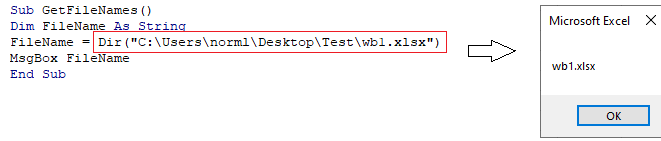
Source: https://trumpexcel.com/vba-dir-function/
Watch my video here
Press Ctrl + Shift + 9 to unhide all rows or Ctrl + Shift + 0 (zero) to unhide all columns. If this doesn't work, then right-click on a row or column identifier and select Unhide.
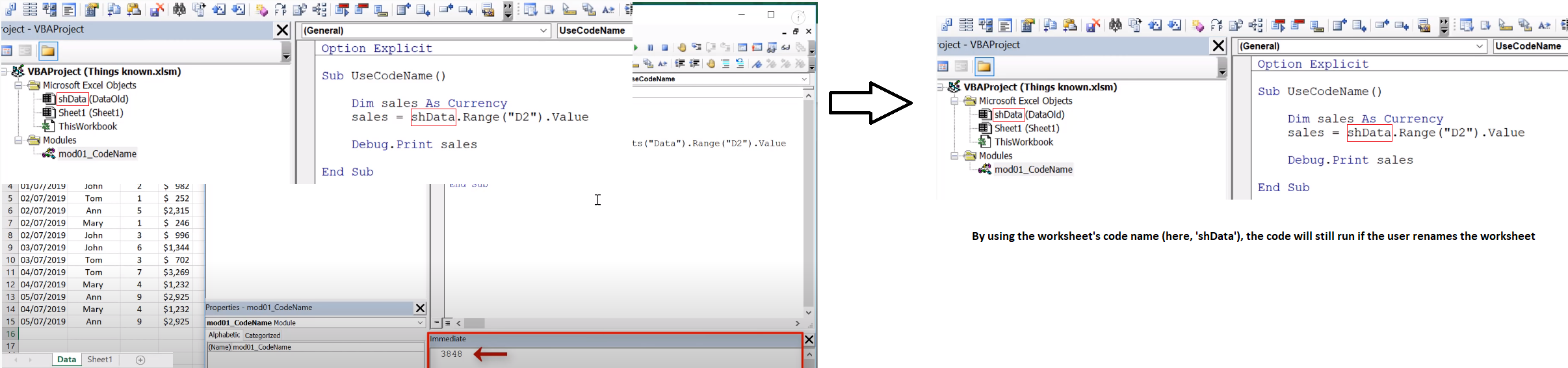
See file here
Sub UseForRangeCopy()
'Get the worksheets
Dim shData As Worksheet, shOutput As Worksheet
Set shData = ThisWorkbook.Worksheets("Data")
Set shOutput = ThisWorkbook.Worksheets("Output")
'Clear any existing data in output sheet
shOutput.Range("A1").CurrentRegion.Offset(1).ClearContents
'Get the range of "Data" worksheet
Dim rg As Range
Set rg = shData.Range("A1").CurrentRegion
'The main code
Dim i As Long, row As Long
row = 2
For i = 2 To rg.Rows.Count
If rg.Cells(i, 4).Value = "Negative" Then
'Copy using selections
'shData.Activate
'rg.Rows(i).Select
'Selection.Copy
'shOutput.Activate
'shOutput.Range("A" & row).Select
'Selection.PasteSpecial xlPasteValues
shOutput.Range("A" & row).Resize(1, rg.Columns.Count).Value = rg.Rows(i).Value
'move to the next output row
row = row + 1
End If
Next i
Application.CutCopyMode = False
End Sub
Press CTRL-F. . .
For counter = initial_value To end_value _
             [Step stepcounter]
'code to execute on each iteration
[Exit For]
Next [counter]
Source: https://www.oreilly.com/library/view/vb-vba/1565923588/1565923588_ch07-1091-fm2xml.html
For Lrow = Lastrow To Firstrow Step -1 'here, Lrow is the counter . . . in this For/Next statement
With .Cells(Lrow, "A")
If Not IsError(.Value) Then
Debug.Print (.Value)
If .Value Like "*xc*" Or .Value Like "* SERVICE:*" Or .Value Like "* Totals*" Then .EntireRow.Delete
'This will delete each row where Column A contains a number
'This will delete each row where Column C contains a number
End If
End With
Next Lrow
To have newline in code you use _
Example:
Dim a As Integer
a = 500 _
  + 80 _
  + 90
Dim LResult

If IsEmpty(LResult) = True Then
Sub askYourName()
Dim yourName As String
yourName = InputBox("What's your name?")
MsgBox ("Your name is " & yourName)
End Sub
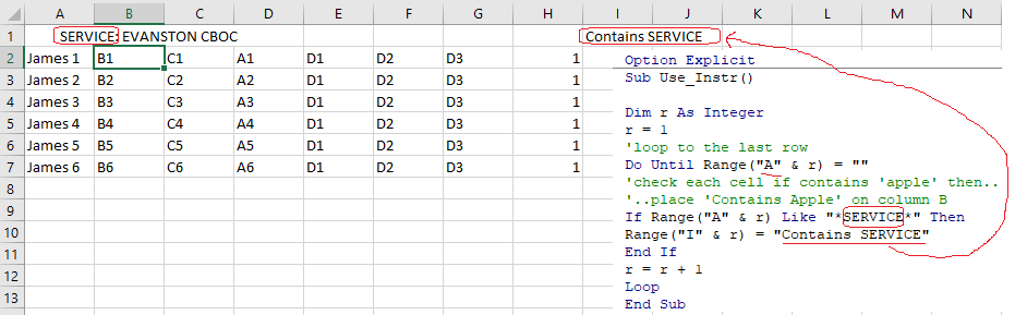 This code loops through column A & looks for any cell that contains "SERVICE" & pastes "Contains SERVICE" onto column I of that row.
Source: https://software-solutions-online.com/excel-vba-if-cell-contains-value-then/
Sub Use_Instr()
R = 1
'loop to the last row
Do Until Range("A" & R) = ""
'check each cell if contains 'apple' then..
'..place 'Contains Apple' on column B
If Range("A" & R) Like "*apple*" Then
Range("B" & R) = "Contains Apple"
End If
R = R + 1
Loop
End Sub
Using LIKE to find cells that contain the word 'Totals' in Sheet 1 & copy those entire rows to Sheet 7
Sub UseForRangeCopy()
'Get the worksheets

Dim shData As Worksheet, shOutput As Worksheet

Set shData = ThisWorkbook.Worksheets("Sheet1")

Set shOutput = ThisWorkbook.Worksheets("Sheet7")
'Clear any existing data in output sheet

shOutput.Range("A1").CurrentRegion.Offset(1).ClearContents
'Get the range of "Data" worksheet

Dim rg As Range

Set rg = shData.Range("A1").CurrentRegion
'The main code

Dim i As Long, row As Long

row = 1

 For i = 1 To rg.Rows.Count
If rg.Cells(i, 1).Value Like "*Totals*" Then
'Copy using selections

            'shData.Activate

            'rg.Rows(i).Select

            'Selection.Copy

            'shOutput.Activate

            'shOutput.Range("A" & row).Select

            'Selection.PasteSpecial xlPasteValues
shOutput.Range("A" & row).Resize(1, rg.Columns.Count).Value = rg.Rows(i).Value
'move to the next output row

row = row + 1
End If

Next i
For . . . each Loop
Video: For . . . each Loop --LinkedIn 2022
 see video here Source: https://stackoverflow.com/questions/33052552/loop-to-go-through-a-list-of-values
Loop: use LEFT fxn to remove characters after a comma
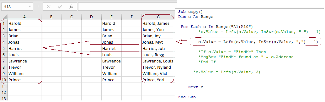 here, the cell values in Column A looked like Column G before running this code . . .
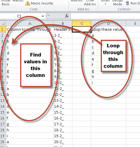
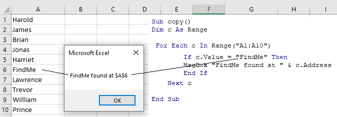
Loop: to find a specific cell value
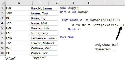
Loop: trim to show only 1st 3 characters
Loop thru a column & Concatenate the Row's values into a sentence -- NL 4.2.22
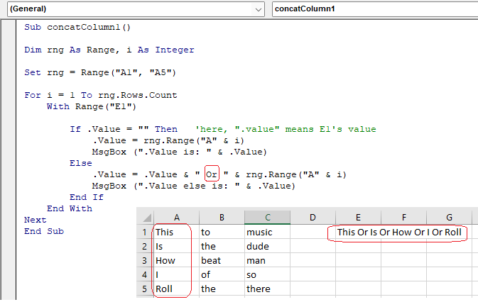
Video: loop thru a column & concatenate rows' values into a sentence in VBA -- NL 4.2.22
Loop thru a column & Concatenate the Row's values (as double quotes) into a sentence -- NL 4.2.22
Video: Loop thru a column & Concatenate the Row's values (as double quotes) into a sentence -- NL 4.2.22
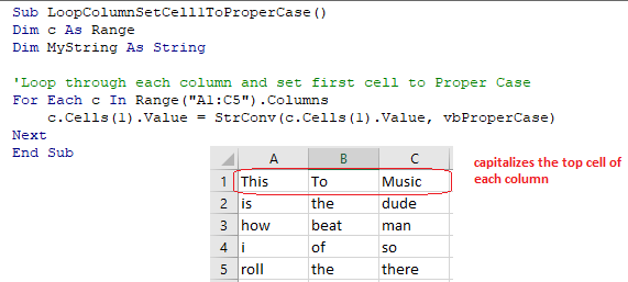
Loop through each column and set first cell to Proper Case
Sub LoopColumn1()
Dim c As Range
Dim MyString As String
'Loop through each column and set first cell to Proper Case
For Each c In Range("A1:C5").Columns
c.Cells(1).Value = StrConv(c.Cells(1).Value, vbProperCase)
Next
End Sub
Video: Loop through each column and set first "top" cell to Proper Case - NL 4.2.22
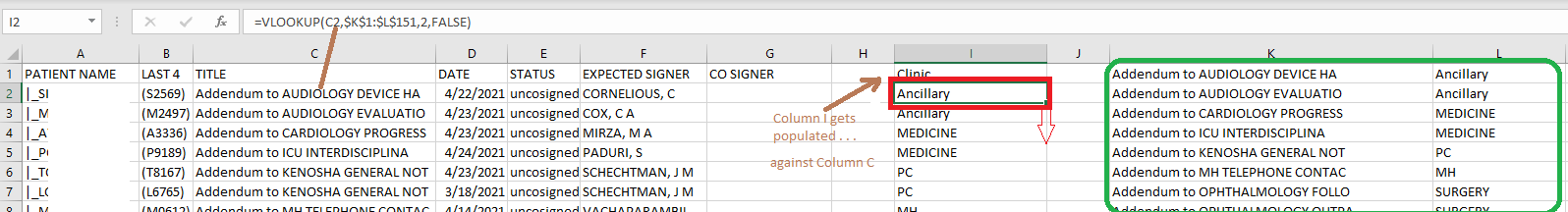
If you are to merge two tables based on one column, VLOOKUP is the right function to use.
Supposing you have two tables in two different sheets: the main table contains the seller names and products, and the lookup table contains the names and amounts. You want to combine these two tables by matching data in the Seller column:
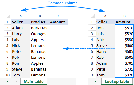
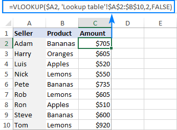
To combine two tables by a matching column (Seller), you enter this formula in C2 in the main table:
=VLOOKUP($A2,'Lookup table'!$A$2:$B$10,2,FALSE)
Where:
Copy the formula down the column, and you will get a merged table consisting of the main table, plus the matched data pulled from the lookup table:
Source: https://www.ablebits.com/office-addins-blog/2018/10/31/excel-merge-tables-matching-columns/
Worksheets("CovidPos").Activate //this activates the "CovidPos" worksheet
b = Worksheets("CovidPos").Cells(Rows.Count, 1).End(xlUp).Row //"b" holds the value for how many rows have data
Worksheets("CovidPos").Cells(b + 1, 1).Select //place cursor on cell that is in row "b + 1" and column 1
ActiveSheet.Paste
See video here
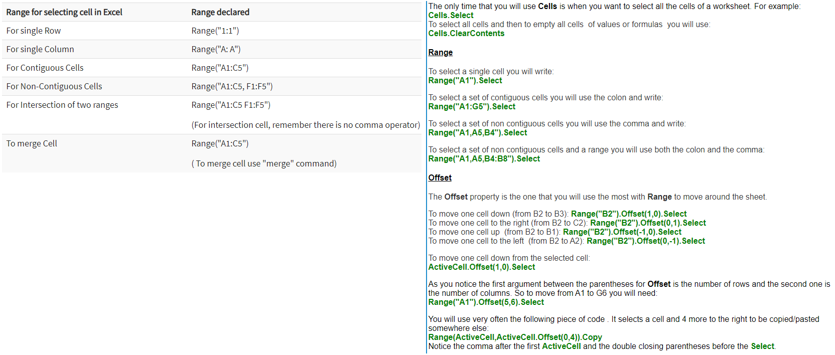
Source: https://www.automateexcel.com/vba/select-range-cells/
Source: https://www.youtube.com/watch?v=DxIzTKgchJ8
Error: Subscript Out of Range
Check to make sure there's not a missing worksheet that's referenced in the VBA code
Error: Runtime Overflow 6
This sounds like you have dimensioned a variable as INTEGER. An integer variable will fail with an OVERFLOW error if it's value exceeds 32767.
DIM your variables as LONG and see if the problem goes away.
Source: https://answers.microsoft.com/en-us/msoffice/forum/msoffice_excel-mso_other-mso_2007/run-time-error-6-overflow-during-macro-run/6a176497-c2b4-44e9-81c1-c921a71a5947
means you have to declare your variables
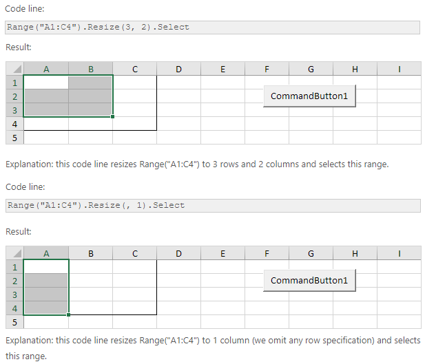
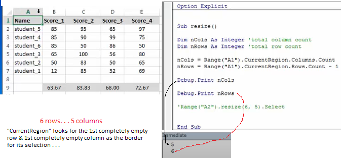
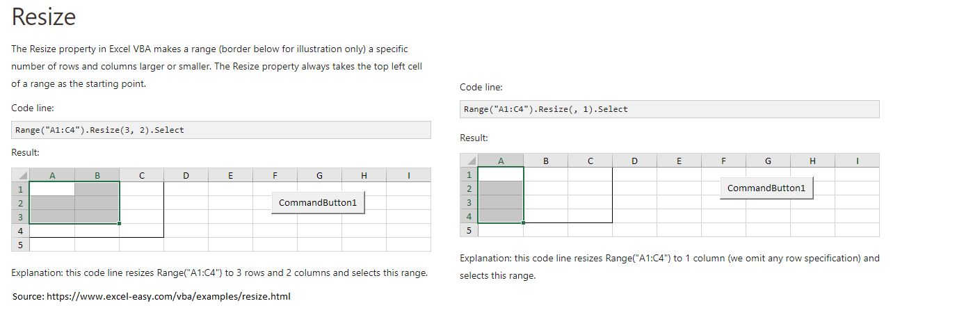
Source: https://www.excel-easy.com/vba/examples/resize.html
Videos:
Using .Resize in Excel 2013 VBA
If the Excel VBA Range object you want to refer to is a single cell, the syntax is simply “Range(“Cell”)”. For example, if you want to make reference to a single cell, such as A1, type “Range(“A1″)”.
Source: https://affordsol.be/vba-code-2-6-cells-ranges.htm
Macro to fill 1st Row with headers from a specific sheet
Sub CopyHeader()
Dim wsSheet As Worksheet
For Each wsSheet In ThisWorkbook.Worksheets
wsSheet.Rows(1).Value = Worksheets("2020").Rows(1).Value ' note that '1' is "one"
Next wsSheet
End Sub
Cells(2, 1).AutoFill Destination:=Range("A2:A2500"), Type:=xlFillSeries
Codename
Sub uoEDmidnightDoD()
Dim a As Long
Dim b As Long
Dim c As Long
Dim marks As String
Dim tally As Long
Dim numRows As Long
Dim lastrow As Long
Dim lastRow0 As Long
Dim lastRow1 As Long
Dim lastRow2 As Long
Dim n As Integer
Dim shData As Worksheet, shOutput As Worksheet
Worksheets.Add.Name = "EMERGENCY CARE DOD MIDNIGHT"
Set shData = ThisWorkbook.Worksheets("2020")
Set shOutput = ThisWorkbook.Worksheets("EMERGENCY CARE DOD MIDNIGHT")
shOutput.Range("A1").CurrentRegion.Offset(1).Clear 'this clears BOTH content & formatting
'Get the range of "2020" worksheet
shData.Activate
Dim rg As Range
Set rg = shData.Range("A2").CurrentRegion 'this places you in A5 in 2020 tab & selects area with contiguous data
'The main code
Dim i, row As Long
row = 2 'you'll now start in row of the area that was selected as "CurrentRegion" . . .
For i = 2 To rg.Rows.Count
marks = rg.Cells(i, 7).Value
If marks = "EMERGENCY CARE DOD MIDNIGHT" Then
'Copy using selections
shOutput.Range("A" & row).Resize(1, rg.Columns.Count).Value = rg.Rows(i).Value
'move to the next output row
row = row + 1
End If
Next i
Worksheets("EMERGENCY CARE DOD MIDNIGHT").Activate
With ActiveSheet
numRows = .Cells(.Rows.Count, "B").End(xlUp).row
.Range("T1").Value = numRows - 1
Range("A2", Range("R2").End(xlDown)).Sort Key1:=Range("H2"), Order1:=xlAscending, Header:=xlNo 'sort by column B2--after looking across from A2 to R2
End With
End Sub
Excel File here
Option Explicit
Sub uoEDmidnightDoD()
Dim a As Long
Dim b As Long
Dim c As Long
Dim marks As String
Dim tally As Long
Dim numRows As Long
Dim lastrow As Long
Dim lastRow0 As Long
Dim lastRow1 As Long
Dim lastRow2 As Long
Dim n, i As Integer
Dim myarray()
myarray = Array("red", "green", "blue")
For i = LBound(myarray) To UBound(myarray)
'Next i
Dim shData As Worksheet, shOutput As Worksheet
Worksheets.Add.Name = myarray(i)
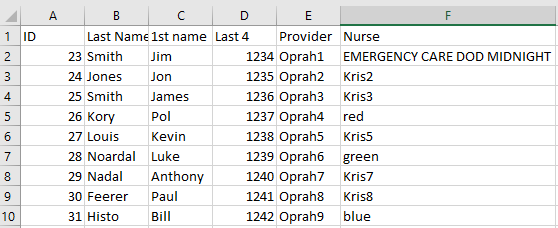
Set shData = ThisWorkbook.Worksheets("Sheet1")
Set shOutput = ThisWorkbook.Worksheets(myarray(i))
shOutput.Range("A1").CurrentRegion.Offset(1).Clear 'this clears BOTH content & formatting
'Get the range of "Sheet1" worksheet
shData.Activate
Dim rg As Range
Set rg = shData.Range("A2").CurrentRegion 'this places you in A2 in Sheet1 tab & selects area with contiguous data
'The main code
Dim j, row As Long
row = 2 'you'll now start in row of the area that was selected as "CurrentRegion" . . .
For j = 2 To rg.Rows.Count
marks = rg.Cells(j, 6).Value
If marks = myarray(i) Then
'Copy using selections
shOutput.Range("A" & row).Resize(1, rg.Columns.Count).Value = rg.Rows(j).Value
'move to the next output row
row = row + 1
End If
Next j
Worksheets(myarray(i)).Activate
With ActiveSheet
numRows = .Cells(.Rows.Count, "B").End(xlUp).row
.Range("T1").Value = numRows - 1
Range("A2", Range("F2").End(xlDown)).Sort Key1:=Range("E2"), Order1:=xlAscending, Header:=xlNo 'sort by column B2--after looking across from A2 to F2
End With
Next i
End Sub
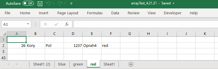
 sheet1
Sub CopyHeader()
Dim wsSheet As Worksheet
For Each wsSheet In ThisWorkbook.Worksheets
wsSheet.Rows(1).Value = Worksheets("2020").Rows(1).Value ' note that '1' is "one"
Next wsSheet
End Sub
Option Explicit
Sub uoDoDClinics()
Dim a As Long
Dim b As Long
Dim c As Long
Dim marks As String
Dim tally As Long
Dim numRows As Long
Dim lastrow As Long
Dim lastRow0 As Long
Dim lastRow1 As Long
Dim lastRow2 As Long
Dim n, i As Integer
Dim myarray()
myarray = Array("1007 AFTER HOURS TREATMENT", "1007 PHYS THERAPY", "AUDIOLOGY NBHC 1523", "CHAMPUS SUPPORT 200H")
For i = LBound(myarray) To UBound(myarray)
'Next i
Dim shData As Worksheet, shOutput As Worksheet
Worksheets.Add.Name = myarray(i)
Set shData = ThisWorkbook.Worksheets("2020")
Set shOutput = ThisWorkbook.Worksheets(myarray(i))
shOutput.Rows(1).Value = shData.Rows(1).Value
shOutput.Columns("A:R").AutoFit
shOutput.Range("A1").CurrentRegion.Offset(1).Clear 'this clears BOTH content & formatting
'Get the range of "Sheet1" worksheet
shData.Activate
Dim rg As Range
Set rg = shData.Range("A2").CurrentRegion 'this places you in A2 in 2020 tab & selects area with contiguous data
'The main code
Dim j, row As Long
row = 2 'you'll now start in row of the area that was selected as "CurrentRegion" . . .
For j = 2 To rg.Rows.Count
marks = rg.Cells(j, 7).Value
If marks = myarray(i) Then
'Copy using selections
shOutput.Range("A" & row).Resize(1, rg.Columns.Count).Value = rg.Rows(j).Value
'move to the next output row
row = row + 1
End If
Next j
Worksheets(myarray(i)).Activate
With ActiveSheet
numRows = .Cells(.Rows.Count, "B").End(xlUp).row
.Range("T1").Value = numRows - 1
Range("A2", Range("R2").End(xlDown)).Sort Key1:=Range("H2"), Order1:=xlAscending, Header:=xlNo 'sort by column H2--after looking across from A2 to R2
End With
Next i
End Sub
Go to page
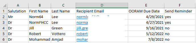
 sends reminder if Column D looks like an email address AND if Column F = "yes"
Access Excel file here
Option Explicit
Sub CreateReminder()
Dim cell As Range
Dim OutApp, OutMail As Object
For Each cell In Sheets("Sheet1").Columns("D").Cells.SpecialCells(xlCellTypeConstants)
If cell.Offset(0, 2).Value <> "" Then 'offsets 2 columns to the right from column D
If cell.Value Like "?*@?*.?*" And LCase(cell.Offset(0, 2).Value) = "yes" Then
Set OutApp = CreateObject("Outlook.Application") 'Create Outlook Application
Set OutMail = OutApp.CreateItem(0) 'Create Email
With OutMail
.to = cell.Value
.Subject = "OORAM Reminder"
.Body = "Dear " & cell.Offset(0, -3).Value & " " & cell.Offset(0, -2).Value & " " & cell.Offset(0, -1).Value & _
":" & vbNewLine & vbNewLine & _
"Reminder: Your OORAM is expiring in 30 days! Please contact Dr Amin Nadeem, Mark Bisbee, or me to schedule the simulation portion. Don't forget to complete the TMS online training (TMS course -VA 16087 Or TMS course -VA 19361) PRIOR to the simulation portion." & vbNewLine & vbNewLine & _
"Thanks!" & vbNewLine & vbNewLine & _
"R," & vbNewLine & _
"N Lee, MD" & vbNewLine & _
"Assistant Chief Medical Executive, Chief Medical Informatics Officer" & vbNewLine & _
"Lovell FHCC" & vbNewLine & _
"Cell: 847-343-1015"
.Attachments.Add "C:\data\FHCC_OOORAM_Template_Reappointment-edit9.3.18.docx"
'.Display 'To send without Displaying change .Display to .Send
.Send
End With
End If
End If
Next cell
End Sub
Source:
Sending Reminder from Excel Using Gmail with CDO --Dinesh Kumar Takyar
Notes:
Google made the SMTP server available only for G Suite customers . . . so can't for-free do automate email reminders using Gmail . . . see Hanshima's reply to YouTube video: https://www.youtube.com/watch?v=cOhupIT0rNA
Source: site here
'COUNTA" means to count all of the rows that have text . . .
Source:
Video: How To Create Custom Word Documents From Excel WITHOUT Mail Merge important timestamps: 6:19 ["days since"]; 7:20 [named dynamic range]; 10:21 ["match"]
Private Sub CommandButton1_Click()
Dim marks As Integer
Dim marks1 As Double
Dim marks2 As Double
Dim marks3, marks4 As Double
Dim sValue As String
Dim marks1decnum As Variant
a = Worksheets("REAL").Cells(Rows.Count, 1).End(xlUp).Row
For i = 2 To a
marks = Worksheets("REAL").Cells(i, 7).Value
marks1 = Worksheets("REAL").Cells(i, 8).Value
marks1decnum = CDec(marks1)
marks2 = Worksheets("REAL").Cells(i, 10).Value
marks2decnum = CDec(marks2)
marks3 = 9.57
marks4 = 26.54
'If marks < 65 And marks1 < Worksheets("REAL").Range("H2").Value And marks2 < Worksheets("REAL").Range("J2").Value Then
'If marks < 65 And marks1 < 12 And marks2 < 33 Then
If marks1decnum <= marks3 And marks2decnum <= marks4 Then
Worksheets("REAL").Rows(i).Copy
Worksheets("Sheet8").Activate
b = Worksheets("Sheet8").Cells(Rows.Count, 1).End(xlUp).Row
Worksheets("Sheet8").Cells(b + 1, 1).Select
ActiveSheet.Paste
Worksheets("REAL").Activate
End If
Next
Application.CutCopyMode = False
ThisWorkbook.Worksheets("REAL").Cells(1, 1).Select
End Sub
Excel workbook here
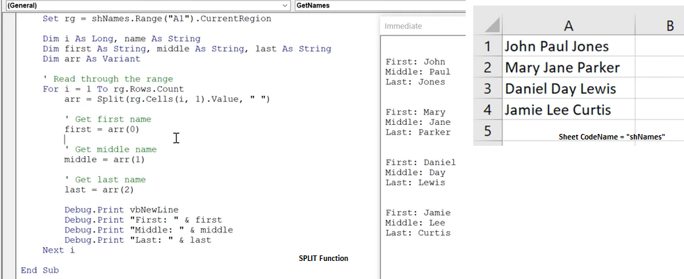
Sub vba_string_array()
Dim myArray() As String
myArray = Split("Today is a good day", " ")
For i = LBound(myArray) To UBound(myArray)
Debug.Print myArray(i)
Next i
End Sub
Video: Using Split() function to separate words in a sentence into an array - NL 4.2.22
The syntax for the SPLIT function in Microsoft Excel is:
Split ( expression [,delimiter] [,limit] [,compare] )
Let's look at some Excel SPLIT function examples and explore how to use the SPLIT function in Excel VBA code:
Split("Tech on the Net")
Result: {"Tech", "on", "the", "Net"}

Split("172.23.56.4", ".")
Result: {"172", "23", "56", "4"}

Split("A;B;C;D", ";")
Result: {"A", "B", "C", "D"}

Split("A;B;C;D", ";", 1)    'this splits the expression into "1" piece within the double quotes
Result: {"A;B;C;D"}

Split("A;B;C;D", ";", 2)   'this splits the expression into "2" pieces
Result: {"A", "B;C;D"}

Split("A;B;C;D", ";", 3)   'this splits the expression into "3" pieces
Result: {"A", "B", "C;D"}

Split("A;B;C;D", ";", 4)    'this splits the expression into "4" pieces, each within double quotes
Result: {"A", "B", "C", "D"}
Video: Convert Values to Uppercase [1st row of each column] -- NL 4.2.22
article here
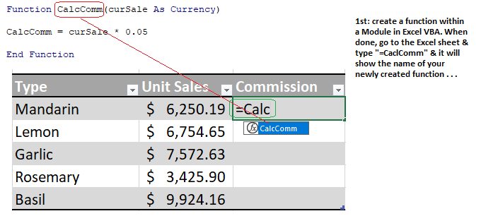
Use functions with VBA
Excel object variables: e.g., Worksheets, Cells, Ranges, etc. For example, Cells.Value (here, "Cells" is the object calling the method "Value"--mine)
Video: Object Variables: Define & Use (LinkedIn 2022)
Example:
Dim WSO as Worksheet
Set WSO = Activesheet
WSO.Copy
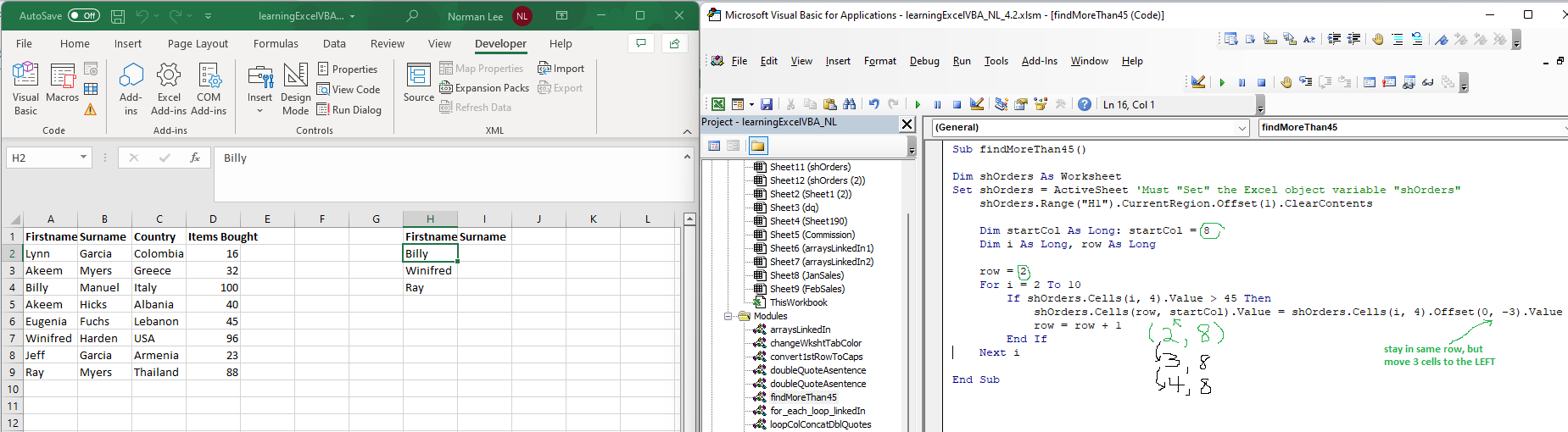
Video: Find > 45, place 1st name into cell - NL 4.4.22
Video: Find > 45, place 1st name into cell - NL 4.4.22
Video: filterBoldColorHighlightSort_4.9.22_NL.mp4
Sub compareColumns()

   ' im assuming the sheet in question is the  index 1 sheet in the workbook
   Dim ws As Worksheet: Set ws = ThisWorkbook.Sheets(1)

   ' im assuming no header
   Dim lastRowA As Integer: lastRowA = ws.Cells(ws.Rows.Count, 1).End(xlUp).Row
   Dim lastRowB As Integer: lastRowB = ws.Cells(ws.Rows.Count, 2).End(xlUp).Row

   Dim i As Integer, j As Integer
   Dim matchMe As String
   For i = 1 To lastRowA
       matchMe = ws.Cells(i, 1).Value

       For j = 1 To lastRowB
           If ws.Cells(j, 2).Value = matchMe Then
               ws.Cells(i, 1).Interior.Color = vbRed
               Exit For
           End If
       Next j
   Next i
End Sub
Source: https://stackoverflow.com/questions/71380856/check-if-value-exists-in-another-column-and-highlight-in-vba
Sub DeleteRows()
Dim c As Range
Dim SrchRng

Set SrchRng = ActiveSheet.Range("A1", ActiveSheet.Range("A65536").End(xlUp))
Do
     Set c = SrchRng.Find("Dog","Cat" LookIn:=xlValues)
     If Not c Is Nothing Then c.EntireRow.Delete
Loop While Not c Is Nothing
End Sub
Source: https://forum.ozgrid.com/forum/index.php?thread/57641-delete-entire-row-if-cell-in-column-contains-certain-text/
Sub Test1()
With Range("A1")
.Value = Date
.NumberFormat = "mm/dd/yy"
End With
End Sub
Source: https://www.mrexcel.com/board/threads/enter-current-date-into-cell-with-vba.130840/
Range("A" & Rows.Count).End(xlUp).Offset(1).Select
Source: https://www.teachexcel.com/excel-tutorial/find-the-next-blank-row-with-vba-macros-in-excel_1261.html
Source: https://software-solutions-online.com/next-without-for-compile-error-in-excel-vba-what-does-it-mean-and-how-do-you-fix-it/
Use Python Pandas in Visual Studio
import pandas as pd
from pandas import ExcelWriter
excel_file_path = r'C:\Users\norml\Pictures\VA\unsignedNotes2022\unsignedORDERS\abridgedDB_unsignedOrdersPlain1.xlsx'
df = pd.read_excel(excel_file_path)
split_values = df['PATIENT LOCATION'].unique()
print(split_values)
output_file = 'unsignedOrd_output.xlsx'
writer = pd.ExcelWriter(output_file, engine='xlsxwriter')
for valueNL in split_values:
df1 = df[df['PATIENT LOCATION'] == valueNL]
df1.to_excel(writer, sheet_name= str(valueNL), index=False)
writer.save()
Below code takes forever . . .
Option Explicit 'use with file: filteredTabsUnsignedOrdersDoDClinics2020_test1_complete.xlsm
Sub uoDoDClinics()
Dim a As Long
Dim b As Long
Dim c As Long
Dim marks As String
Dim tally As Long
Dim numRows As Long
Dim lastrow As Long
Dim lastRow0 As Long
Dim lastRow1 As Long
Dim lastRow2 As Long
Dim n, i As Integer
Dim myarray()
myarray = Array("1007 AFTER HOURS TREATMENT", "1007 PHYS THERAPY", "AUDIOLOGY NBHC 1523", "CHAMPUS SUPPORT 200H", _
"COMMITMENT (BLUE) 1007", "COURAGE (WHITE) 1007", "DENTAL BMC 1017 SUPPORT", "DENTAL SERVICE 1017", _
"DENTAL SERVICE 237", "DFM RESPIRATORY COVID19 CLINIC", "DOD MILITARY BLOOD PROGRAM", "EKG - DVC PLACEMENTREMOVAL", _
"FAM MED PCMH TEAM 1", "FEMALE SCREENING 1523", "IMMUNIZATION 1523", "IMMUNIZATION NBHC 237", "INT MED PCMH TEAM 1", _
"LABORATORY 200H", "LABORATORY BMC 1007", "LABORATORY BMC 1523", "LABORATORY NBHC 237", "MED. ASSESSMENT1523", _
"OCC HLTH CLINIC NBHC 237", "OPERATIONAL MEDICINE NBHC 237", "PHARMACY--DENTAL 1017", "PODIATRY CLINIC NBHC 1007", _
"QQQCHCSIITESTGRTLKS", "RECRUIT REHABILITATION UNIT", "RTC ROM SICK CALL", "SHIP 5 SICKCALL CONSTITUTION", _
"SMART TEAM 1007", "SPECIAL PHYSICALS NBHC 1007", "STAFF MEDICINE NBHC 237", "STAFF MILITARY SICKCALL", _
"STUDENT MEDICINE NBHC 237", "USS TRANQUILLITY", "UTILIZATION MANAGEMENT", "WEEKEND MIL. SICK CALL 1007", _
"WELLNESS CLINIC FEMALE")
For i = LBound(myarray) To UBound(myarray)
'Next i
Dim shData As Worksheet, shOutput As Worksheet
Worksheets.Add.Name = myarray(i)
Set shData = ThisWorkbook.Worksheets("2020")
Set shOutput = ThisWorkbook.Worksheets(myarray(i))
shOutput.Rows(1).Value = shData.Rows(1).Value
shOutput.Columns("A:R").AutoFit
shOutput.Range("A1").CurrentRegion.Offset(1).Clear 'this clears BOTH content & formatting
'Get the range of "Sheet1" worksheet
shData.Activate
Dim rg As Range
Set rg = shData.Range("A2").CurrentRegion 'this places you in A2 in 2020 tab & selects area with contiguous data
'The main code
Dim j, row As Long
row = 2 'you'll now start in row of the area that was selected as "CurrentRegion" . . .
For j = 2 To rg.Rows.Count
marks = rg.Cells(j, 7).Value 'I chose 7 because column G is what I need
If marks = myarray(i) Then
'Copy using selections
shOutput.Range("A" & row).Resize(1, rg.Columns.Count).Value = rg.Rows(j).Value
'move to the next output row
row = row + 1
End If
Next j
Worksheets(myarray(i)).Activate
With ActiveSheet
numRows = .Cells(.Rows.Count, "B").End(xlUp).row
.Range("T1").Value = numRows - 1
Range("A2", Range("R2").End(xlDown)).Sort Key1:=Range("H2"), Order1:=xlAscending, Header:=xlNo 'sort by column H2--after looking across from A2 to R2
End With
Next i
End Sub
import pandas as pd
import openpyxl, pprint #make sure you've: pip install xlrd to be able to use the method 'read_excel()'
#read the excel data
xlsx_source = 'manyLocs.xlsx' #don't forget to copy this file into your Visual Studio Python Project folder!
df = pd.read_excel(xlsx_source, sheet_name=0, header=0) #header=0 means that the headers are in the 1st row
df_apples = df[(df['PATIENTLOCATION'] == 'DOD MILITARY BLOOD PROG') | (df['PATIENTLOCATION'] == 'LABORATORY NBHC 237') ]
#create excel
df_apples.to_excel('receivingFile2.xlsx', sheet_name='DoDMBP') #| (df['PATIENTLOCATION'] == 'LABORATORY NBHC 237')
***************
Combine Certain Sheets into a New Worksheet
import pandas as pd
import openpyxl, pprint #make sure you've: pip install xlrd to be able to use the method 'read_excel()'
#read the excel data
xlsx_source = 'manyLocs.xlsx'
#df = pd.read_excel(xlsx_source, sheet_name=0, header=0) #header=0 means that the headers are in the 1st row
#df_apples = df[(df['PATIENTLOCATION'] == 'DOD MILITARY BLOOD PROG') | (df['PATIENTLOCATION'] == 'LABORATORY NBHC 237') ]
#create excel
#df_apples.to_excel('receivingFile2.xlsx', sheet_name='DoDMBP')
df1 = pd.read_excel(xlsx_source, "Sheet1")
df2 = pd.read_excel(xlsx_source, "Sheet2")
# concat both DataFrame into a single DataFrame
df = pd.concat([df1, df2], axis=0) #a zero means to stack the results on top of each other
# Export Dataframe into Excel file
df.to_excel('final_output.xlsx', index=False)
import pandas as pd
import openpyxl, pprint
xlsx_source = 'testMergeSheets1a.xlsx' 'make sure it's an 'xlsx' file type and make sure the headers are all the same across All sheets
excel_file = pd.read_excel(xlsx_source, sheet_name=None, header=0)
dataset_combined = pd.concat(excel_file.values())
dataset_combined.to_excel('dataset_combined.xlsx', index=False) 'source: https://www.youtube.com/watch?v=yKsqn3JN4Qg
VistA: ^Text --> 1 --> 6 --> ALL --> 1/1/21 to t - 1 --> ALL --> Full --> Capture Setup --> Disk --> Browse --> Desktop --> "todays date" --> Save --> OK --> Start Capture --> click 132; --> ;132;99999999999 --> Enter --> Enter --> Enter
Open Excel Macro-enabled Sheet --> run deleteSheetsExcept module --> rename "Data" sheet to "DataOld"
Double click to open the .txt file using Notepad: Ctrl-A, Ctrl-C --> open blank sheet in Excel & straight paste into a sheet
Run deleteSpecificRows module on this active sheet
Stretch Column A across; move Column A to Column C
In tab "equivGroupSorted", column Column A and paste into Column A of Active Sheet
Edit: "Service: Medicine" to "Service: Medicine0" --this is Primary Care's "Medicine"
Remove slashes
Rename new sheet as "Data"
Create new Column B in sheet named "CountsByClinic"
After running "match_range_copy_works_41722" module: Delete DataOld sheet
Save a non-macro copy to run in Pandas
#Ancillary: AUDIOLOGSPEECH PATH., IMAGING SERVICE, LABORATORY SERVICE, NUTRITION AND FOOD SERVICE, OPTOMETRY SECTION,
#PHARMACY SERVICE, PHYSICAL THERAPY, PROSTHETICS & SENSORY AID, RADIOLOGY SECTION, REHABILITATION,
#CLC-HCBC: GERIATRICS & EXTENDED CARE, HOME COMMUNITY BASED CARE, COMMUNITY LIVING CENTER
#CME-CmdSte: CHIEF MEDICAL EXECUTIVE, COMMAND SUITE, INFECTION CONTROL, OCC DELIVERY OPS, OFFICE OF PERFORMANCE IMP
#Dental: ASSOCIATE DIR DENTAL SERVICES, DENTAL
#Facilities: FACILITY MANAGEMENT SERVICE
#Fleet: ASSOCIATE DIR FLEET MEDICINE, FISHER BRANCH CLINIC - 237, OCCUPATIONAL HEALTH MEDICINE, USS TRANQUILITY - 1007
#Inpatient & ICU: ACUTE INPATIENT, CRITICAL CARE SECTION, INPATIENT ACUTE CARE & ICU, INPATIENT SERVICES
#Medicine: CARDIOLOGY SECTION, DERMATOLOGY SECTION, EMERGENCY DEPARTMENT, ENDOCRINOLOGY SECTION, GASTROENTEROLOGY SECTION,
#INFECTIOUS DISEASE SECTION, MEDICAL SERVICE, MEDICAL SERVICES, MEDICINE, Medicine Services, MEDICINE0,
#NEPHROLOGY SECTION, NEUROLOGY SERVICE, PULMONARY DISEASE SECTION, PULMONARY DISEASE SECTION0,
#SPECIAL MEDICAL EXAMS, SPECIAL PROGRAMS, SPECIALTY MEDICINE
#Mental Health: DOMICILIARY SERVICE, MENTAL HEALTH CLINIC, MENTAL HEALTH SERVICE, MENTAL HEALTH TEAM A, SARPATP, SOCIAL WORK
#Nursing: NURSING SERVICE
#PC: EVANSTON CBOC, INTERNAL MEDICINE, KENOSHA CLINIC, PATIENT ALIGNED CARE TEAM, PEDIATRICS, PRIMARY CARE DIR (MHPPACT),
#WOMEN'S PRIMARY CARE
#PtAdmin: EDUCATION, HEALTH CARE BUSINESS, MADISON TELEPHONE OPERATIONS, OUTPATIENTCONSULTATION,
#PATIENT ADMINISTRATION SERVICE, REMOTE, RESOURCES MANAGEMENT, ROCKFORD, UNKNOWN, VISTA APPLICATIONS SUPPORT
#Surgery: GENERAL SURGERY, OPERATING ROOM, OPHTHALMOLOGY SECTION, ORTHOPEDIC SECTION, PODIATRY SECTION,
#Surgery, SURGICAL SERVICE, UROLOGY
"ACUTE INPATIENT", "ASSOCIATE DIR DENTAL SERVICES", "ASSOCIATE DIR FLEET MEDICINE", "AUDIOLOGSPEECH PATH.", "CARDIOLOGY SECTION", "CHIEF MEDICAL EXECUTIVE", "COMMAND SUITE", "COMMUNITY LIVING CENTER", "CRITICAL CARE SECTION", "DENTAL", "DERMATOLOGY SECTION", "DOMICILIARY SERVICE", "EDUCATION", "EMERGENCY DEPARTMENT", "ENDOCRINOLOGY SECTION", "EVANSTON CBOC", "FACILITY MANAGEMENT SERVICE", "FISHER BRANCH CLINIC - 237", "GASTROENTEROLOGY SECTION", "GENERAL SURGERY", "GERIATRICS & EXTENDED CARE", "HEALTH CARE BUSINESS", "HOME COMMUNITY BASED CARE", "IMAGING SERVICE", "INFECTION CONTROL", "INFECTIOUS DISEASE SECTION", "INPATIENT ACUTE CARE & ICU", "INPATIENT SERVICES", "INTERNAL MEDICINE", "KENOSHA CLINIC", "LABORATORY SERVICE", "MADISON TELEPHONE OPERATIONS", "MEDICAL SERVICE", "MEDICAL SERVICES", "MEDICINE", "Medicine Services", "MEDICINE0", "MENTAL HEALTH CLINIC", "MENTAL HEALTH SERVICE", "MENTAL HEALTH TEAM A", "NEPHROLOGY SECTION", "NEUROLOGY SERVICE", "NURSING SERVICE", "NUTRITION AND FOOD SERVICE", "OCC DELIVERY OPS", "OCCUPATIONAL HEALTH MEDICINE", "OFFICE OF PERFORMANCE IMP", "OPERATING ROOM", "OPHTHALMOLOGY SECTION", "OPTOMETRY SECTION", "ORTHOPEDIC SECTION", "OUTPATIENTCONSULTATION", "PATIENT ADMINISTRATION SERVICE", "PATIENT ALIGNED CARE TEAM", "PEDIATRICS", "PHARMACY SERVICE", "PHYSICAL THERAPY", "PODIATRY SECTION", "PRIMARY CARE DIR (MHPPACT)", "PROSTHETICS & SENSORY AID", "PULMONARY DISEASE SECTION", "PULMONARY DISEASE SECTION0", "RADIOLOGY SECTION", "REHABILITATION", "REMOTE", "RESOURCES MANAGEMENT", "ROCKFORD", "SARPATP", "SOCIAL WORK", "SPECIAL MEDICAL EXAMS", "SPECIAL PROGRAMS", "SPECIALTY MEDICINE", "Surgery", "SURGICAL SERVICE", "UNKNOWN", "UROLOGY", "USS TRANQUILITY - 1007", "VISTA APPLICATIONS SUPPORT", "WOMEN'S PRIMARY CARE"
Sub copyDataToNewSheet()
Dim copySheet As Worksheet
Dim pasteSheet As Worksheet
Set copySheet = Worksheets(" ASSOCIATE DIR DENTAL SERVICES")
Set pasteSheet = Worksheets("merged1")
copySheet.Activate
Range("A1").CurrentRegion.Select
Selection.Copy
pasteSheet.Cells(Rows.Count, 1).End(xlUp).Offset(1, 0).PasteSpecial xlPasteValues
Application.CutCopyMode = False
End Sub
Using Arrays. . .
Option Explicit
Sub copyDataToNewSheet()
Dim shData As Worksheet
Dim shOutput As Worksheet
Dim myarray()
Dim i As Long
myarray = Array(" ASSOCIATE DIR DENTAL SERVICES", " DENTAL")
For i = LBound(myarray) To UBound(myarray)
Set shData = ThisWorkbook.Worksheets(myarray(i))
Set shOutput = ThisWorkbook.Worksheets("DentalMerged") 'the output sheet is named "merged1"--don't forget to create this before running this code!
shData.Activate
Dim rg As Range
Set rg = shData.Range("A1").CurrentRegion
shData.Range("A1").CurrentRegion.Select
Selection.Copy
shOutput.Cells(Rows.Count, 1).End(xlUp).Offset(1, 0).PasteSpecial xlPasteValues
Application.CutCopyMode = False
shOutput.Activate
Next i
End Sub
Videos:
Copy Data to another Excel workbook based on sales and date criteria using VBA (youtube.com) Dinesh
Columns("A:B").EntireColumn.AutoFit
Source: https://stackoverflow.com/questions/24058774/excel-vba-auto-adjust-column-width-after-pasting-data
Font PropertiesWorksheets("Sheet1").Range("A1").Font.Color = vbRed
Worksheets("Sheet1").Range("A1").Font.Color = RGB(255, 0, 0)
Worksheets("Sheet1").Range("A1").Font.Color = -16776961
Worksheets("Sheet1").Range("A1").Font.Bold = True
Source: https://www.excel-easy.com/vba/examples/font.html
Sub findUniques()
Dim shData As Worksheet, shOutput As Worksheet
Set shData1 = ThisWorkbook.Worksheets("Sheet15")
shData1.Range("A1:A659").AdvancedFilter Action:=xlFilterCopy, CopyToRange:=Range("B1"), Unique:=True 'prints uniques from Column A's list to Column B
End Sub
Source: https://stackoverflow.com/questions/36044556/quicker-way-to-get-all-unique-values-of-a-column-in-vba
Also----
If data are in column A, then in B1, type in: =UNIQUE(A1:Axx)
or, if you want it sorted alphabetically, type in: =UNIQUE(SORT(A1:Axx))
Sub test()
    Dim ws As Worksheet
    Set ws = ThisWorkbook.Worksheets("Mysheet")
    ws.Columns("A:S").EntireColumn.AutoFit
End Sub
Sub SortWorksheetsTabs()
Application.ScreenUpdating = False
Dim ShCount As Integer, i As Integer, j As Integer
ShCount = Sheets.Count
For i = 1 To ShCount - 1
For j = i + 1 To ShCount
If UCase(Sheets(j).Name) < UCase(Sheets(i).Name) Then
Sheets(j).Move before:=Sheets(i)
End If
Next j
Next i
Application.ScreenUpdating = True
End Sub
Source: https://trumpexcel.com/sort-worksheets/
Option Explicit
Sub practiceOffset()
Dim from As Worksheet: Set from = ThisWorkbook.Sheets("from")
Dim toe As Worksheet: Set toe = ThisWorkbook.Sheets("toe")
'from.Range("A5:B5").Copy Worksheets("toe").Cells(Rows.Count, 1).End(xlUp)
'from.Range("A5:B5").Copy Worksheets("toe").Cells(Rows.Count, 1).End(xlUp)(2) 'pastes to row below last row with values
from.Range("A5:B5").Copy Worksheets("toe").Cells(Rows.Count, 1).End(xlUp)(2).Offset(1, 0) 'pastes to cell 2 rows below the last row that has values
End Sub
What is (2)? It offsets the resulting row by the Number (including the original row)
So if
Worksheets("Name").Cells(Rows.Count, 1).End(xlUp) = A10
typing in "(2)" will offset that by 2 rows (including row 10), so it goes to Row 11
Worksheets("Name").Cells(Rows.Count, 1).End(xlUp)(2) = A11
Source: https://www.mrexcel.com/board/threads/end-xlup-2.336210/
Range("A1:I" & Range("A1").End(xlDown).Row).Select or. . .
Sub hfjksaf()
Dim N As Long
N = Cells(1, 1).End(xlDown).Row
Range("A1:I" & N).Select
End Sub
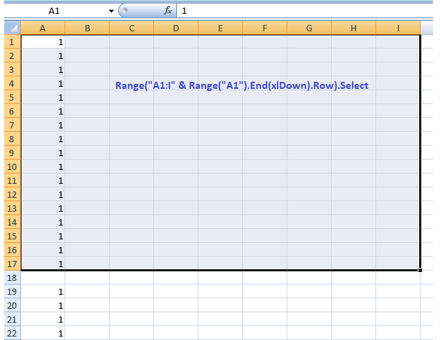
Source: https://stackoverflow.com/questions/28306140/select-cells-in-range-until-row-is-blank
LastRow = Cells(Rows.Count, "B").End(xlUp).Row + 1
Option Explicit
Sub Lastrow()

Dim Lastrow As Long

Lastrow = Cells(Rows.Count, "B").End(xlUp).Row + 1

MsgBox Lastrow

Range("B" & Lastrow & ":M" & Lastrow).Merge

End Sub
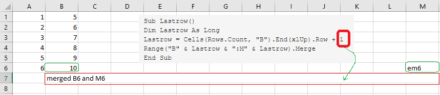
Source: https://www.mrexcel.com/board/threads/selecting-cells-below-last-row-of-worksheet.942747/
Option Explicit
Sub findLastRow()
Dim lastRow As Long
Dim lastRowAddress As Variant
lastRow = Sheets("from").Range("A99999").End(xlUp).Row
lastRowAddress = Sheets("from").Range("A99999").End(xlUp).Address
MsgBox lastRow
MsgBox lastRowAddress
End Sub
or . . .
Sub findLastRow1()
Dim lastRow As Long
Dim lastRowAddress As Variant
lastRow = Sheets("from").Cells(Rows.Count, 1).End(xlUp).Row 'note that we can't use Range object, need to use Cells object
lastRowAddress = Sheets("from").Cells(Rows.Count, 1).End(xlUp).Address
MsgBox lastRow
MsgBox lastRowAddress
End Sub
Source: https://www.youtube.com/watch?v=QPhk3W6C0vk
Sub countrows1()
Dim X As Integer
X = Range("D4:D11").Rows.Count
MsgBox "Number of used rows is " & X
End Sub
Source: https://www.exceldemy.com/excel-vba-count-rows-with-data-in-column/
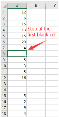
Copy range of cells in column until blank cell, and paste into new worksheetOption Explicit
Sub matchFilterMay4() 'use with Excel file http://www.medical-life-skills.com/Contents/VBA/FHCC_works/toTest_5.5.22_0633.xlsm
' using sheet named "Data" in the workbook
Dim ws As Worksheet: Set ws = ThisWorkbook.Sheets("Data")
' im assuming no header
' remove Dim lastRowA As Integer: lastRowA = ws.Cells(ws.Rows.Count, 1).End(xlUp).Row '1 means column A
Dim lastRowC As Integer: lastRowC = ws.Cells(ws.Rows.Count, 3).End(xlUp).Row '3 means column C
Dim i As Integer, j As Integer, k As Integer
Dim startRow As Long
Dim matchMe As String, newString As String, marks As String
Dim myarray As Variant
myarray = Array("SERVICE: EVANSTON CBOC", "SERVICE: ASSOCIATE DIR DENTAL SERVICES", "SERVICE: ASSOCIATE DIR FLEET MEDICINE", _
"SERVICE: AUDIOLOGSPEECH PATH.", "SERVICE: CARDIOLOGY SECTION", "SERVICE: CHIEF MEDICAL EXECUTIVE", "SERVICE: COMMAND SUITE", _
"SERVICE: COMMUNITY LIVING CENTER", "SERVICE: CRITICAL CARE SECTION", "SERVICE: DENTAL", "SERVICE: DERMATOLOGY SECTION", _
"SERVICE: DOMICILIARY SERVICE", "SERVICE: EDUCATION", "SERVICE: EMERGENCY DEPARTMENT", "SERVICE: ENDOCRINOLOGY SECTION", _
"SERVICE: ACUTE INPATIENT", "SERVICE: FACILITY MANAGEMENT SERVICE", "SERVICE: FISHER BRANCH CLINIC - 237", _
"SERVICE: GASTROENTEROLOGY SECTION", "SERVICE: GENERAL SURGERY", "SERVICE: GERIATRICS & EXTENDED CARE", _
"SERVICE: GERIATRICS & EXTENDED CARE0", "SERVICE: HEALTH CARE BUSINESS", "SERVICE: HOME COMMUNITY BASED CARE", _
"SERVICE: IMAGING SERVICE", "SERVICE: INFECTION CONTROL", "SERVICE: INFECTIOUS DISEASE SECTION", _
"SERVICE: INPATIENT ACUTE CARE & ICU", "SERVICE: INPATIENT SERVICES", "SERVICE: INTERNAL MEDICINE", _
"SERVICE: INTERNAL MEDICINE0", "SERVICE: KENOSHA CLINIC", "SERVICE: KENOSHA CLINIC0", "SERVICE: LABORATORY SERVICE", _
"SERVICE: MADISON TELEPHONE OPERATIONS", "SERVICE: MANAGED CARE OPERATIONS", "SERVICE: MEDICAL SERVICE", _
"SERVICE: MEDICAL SERVICES", "SERVICE: MEDICINE", "SERVICE: Medicine Services", "SERVICE: MEDICINE0", _
"SERVICE: MEDICINE1", "SERVICE: MEDICINE2", "SERVICE: MENTAL HEALTH CLINIC1", "SERVICE: MENTAL HEALTH CLINIC", _
"SERVICE: MENTAL HEALTH CLINIC0", "SERVICE: MENTAL HEALTH SERVICE", "SERVICE: MENTAL HEALTH TEAM A", _
"SERVICE: NEPHROLOGY SECTION", "SERVICE: NEUROLOGY SERVICE", "SERVICE: NURSING SERVICE", "SERVICE: NUTRITION AND FOOD SERVICE", _
"SERVICE: OCC DELIVERY OPS", "SERVICE: OCCUPATIONAL HEALTH MEDICINE", "SERVICE: OFFICE OF PERFORMANCE IMP", "SERVICE: OPERATING ROOM", _
"SERVICE: OPHTHALMOLOGY SECTION", "SERVICE: OPTOMETRY SECTION", "SERVICE: ORTHOPEDIC SECTION", "SERVICE: OUTPATIENTCONSULTATION", _
"SERVICE: PATIENT ADMINISTRATION SERVICE", "SERVICE: PATIENT ALIGNED CARE TEAM", "SERVICE: PATIENT ALIGNED CARE TEAM0", _
"SERVICE: PATIENT ALIGNED CARE TEAM1", "SERVICE: PEDIATRICS", "SERVICE: PHARMACY SERVICE", "SERVICE: PHARMACY SERVICE0", _
"SERVICE: PHARMACY SERVICE1", "SERVICE: PHYSICAL THERAPY", "SERVICE: PODIATRY SECTION", "SERVICE: PRIMARY CARE DIR (MHPPACT)", _
"SERVICE: PROSTHETICS & SENSORY AID", "SERVICE: PULMONARY DISEASE SECTION", "SERVICE: PULMONARY DISEASE SECTION0", _
"SERVICE: RADIOLOGY SECTION", "SERVICE: REHABILITATION", "SERVICE: REMOTE", "SERVICE: RESOURCES MANAGEMENT", "SERVICE: ROCKFORD", _
"SERVICE: SARPATP", "SERVICE: SOCIAL WORK", "SERVICE: SPECIAL MEDICAL EXAMS", "SERVICE: SPECIAL PROGRAMS", "SERVICE: SPECIALTY MEDICINE", _
"SERVICE: Surgery", "SERVICE: SURGICAL SERVICE", "SERVICE: UNKNOWN", "SERVICE: UROLOGY", "SERVICE: USS TRANQUILITY - 1007", _
"SERVICE: VISTA APPLICATIONS SUPPORT", "SERVICE: WOMEN'S PRIMARY CARE")
Sheets.Add.Name = "MedicineMerged"
For i = LBound(myarray) To UBound(myarray)
For j = 1 To lastRowC
marks = ws.Cells(j, 3).Value
If marks = myarray(i) Then
'ws.Cells(i, 1).Interior.Color = vbRed
'Debug.Print j 'prints matching row number to Immediate window
'newString = Replace(ws.Cells(j, 3).Value, "SERVICE: ", "")
'Worksheets.Add.Name = newString
'Debug.Print newString
'Sheets.Add.Name = newString
Debug.Print ws.Cells(j, 3).Address
Dim Var1 As Range
Dim Var2 As Range, sText As Variant
Set Var1 = ws.Cells(j, 3)
Set Var2 = Var1.End(xlDown)
Debug.Print Var1.Address
Debug.Print Var2.Address
Dim strAddress1 As String, strAddress2 As String
Dim rownum1 As Long, rownum2 As Long
strAddress1 = Var1.Address
strAddress2 = Var2.Address
rownum1 = Range(strAddress1).Row 'yields the row number of the cell's address
rownum2 = Range(strAddress2).Row
Debug.Print rownum1
Debug.Print rownum2
ws.Activate
'ws.Range("C" & rownum1 & ":" & "C" & rownum2).Select
If ws.Range("C" & rownum1 + 1) <> "" Then
ws.Range("D" & rownum1 + 1 & ":" & "D" & rownum2) = ws.Range("C" & rownum1)
'ws.Range("C" & rownum1 & ":" & "C" & rownum2).Copy Worksheets(newString).Range("A1") 'this is the magic
'ws.Range("D" & rownum1 & ":" & "D" & rownum2).Copy Worksheets(newString).Range("B1") 'this is the magic
'ws.Range("C" & rownum1) = "" 'deletes header for clinic section in sheet "Data"
'Worksheets(newString).Columns("A:B").EntireColumn.AutoFit
Dim marks1 As String
marks1 = ws.Range("C" & rownum1).Value
'If ws.Range("C" & rownum1).Value = "SERVICE: GASTROENTEROLOGY SECTION" Then
If marks1 = "SERVICE: GASTROENTEROLOGY SECTION" Or marks1 = "SERVICE: ENDOCRINOLOGY SECTION" _
Or marks1 = "SERVICE: CARDIOLOGY SECTION" Or marks1 = "SERVICE: DERMATOLOGY SECTION" _
Or marks1 = "SERVICE: EMERGENCY DEPARTMENT" Or marks1 = "SERVICE: INFECTIOUS DISEASE SECTION" _
Or marks1 = "SERVICE: MEDICINE" Or marks1 = "SERVICE: MEDICINE0" Or marks1 = "SERVICE: MEDICINE1" _
Or marks1 = "SERVICE: MEDICINE2" Or marks1 = "SERVICE: Medicine Services" Or marks1 = "SERVICE: NEPHROLOGY SECTION" _
Or marks1 = "SERVICE: NEUROLOGY SERVICE" Or marks1 = "SERVICE: PULMONARY DISEASE SECTION" Or marks1 = "SERVICE: PULMONARY DISEASE SECTION0" _
Or marks1 = "SERVICE: SPECIALTY MEDICINE" Then
ws.Range("C" & rownum1 & ":" & "C" & rownum2).Copy Worksheets("MedicineMerged").Cells(Rows.Count, 1).End(xlUp)(2).Offset(1, 0)
Else
Debug.Print "No"
End If
Else
Debug.Print "Else"
End If
Exit For
End If
Next j
Next i
End Sub
Source:https://stackoverflow.com/questions/56981081/copy-range-of-cells-in-column-until-blank-cell-and-paste-into-new-workbook
Option Explicit
Sub findFirstBlankRowFromTop()
Dim x As Integer
Dim NumRows As Long
Application.ScreenUpdating = False
'set numrows = number of rows of data
NumRows = Range("A1", Range("A1").End(xlDown)).Rows.Count
MsgBox NumRows
'select A1
Range("A1").Select
'Establish "For" loop to loop "NumRows" number of times
For x = 1 To NumRows
Debug.Print "loop"
ActiveCell.Offset(1, 0).Select 'this selects the cell below the last selection
Next
Application.ScreenUpdating = True
End Sub
Source: https://www.extendoffice.com/documents/excel/4438-excel-loop-until-blank.html
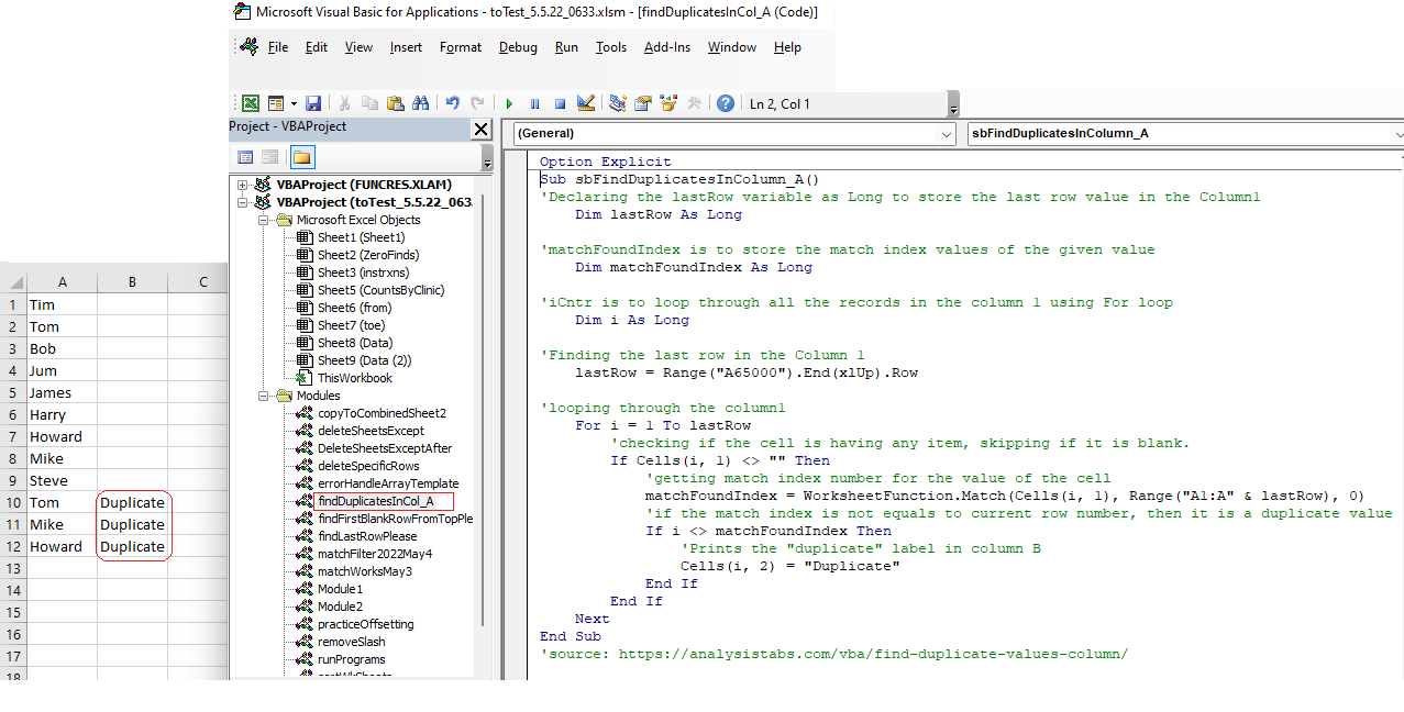
Sub findDuplicatesInColumn_A()
'Declaring the lastRow variable as Long to store the last row value in the Column1
Dim lastRow As Long
'matchFoundIndex is to store the match index values of the given value
Dim matchFoundIndex As Long
'iCntr is to loop through all the records in the column 1 using For loop
Dim i As Long
'Finding the last row in the Column 1
lastRow = Range("A65000").End(xlUp).Row
'looping through the column1
For i = 1 To lastRow
'checking if the cell is having any item, skipping if it is blank.
If Cells(i, 1) <> "" Then
'getting match index number for the value of the cell
matchFoundIndex = WorksheetFunction.Match(Cells(i, 1), Range("A1:A" & lastRow), 0)
'if the match index is not equals to current row number, then it is a duplicate value
If i <> matchFoundIndex Then
'Prints the "duplicate" label in column B
Cells(i, 2) = "Duplicate"
End If
End If
Next
End Sub
'source: https://analysistabs.com/vba/find-duplicate-values-column/
Sub fillTopRows() 'this will fill the tops of ALL worksheets in the Workbook with the contents in the array
Dim xSh As Worksheet
Application.ScreenUpdating = False
For Each xSh In Worksheets
xSh.Select
[A1:G1] = Split("PatientName Last4 Title Date Status ExpectedSigner ExpectedCoSigner") 'make sure there are no gaps in the title headers
xSh.Range("A1:G1").Font.Bold = True
Next
Application.ScreenUpdating = True
End Sub
'don't forget to "fillTheTopRows.fillTopRows" when filling in the button command code
5.2.22:
=RIGHT(S2,LEN(S2)-7)

The above formula uses the LEN function to get the total number of characters in the cell in column A.
From the value that we get from the LEN function, we subtract 3, as we only want to extract the numbers and want to remove the first three characters from the left of the string in each cell.
This value is then used within the RIGHT function to extract everything except the first three characters from the left.
This code will insert the new sheet AFTER another sheet named "Input":
|
Sheets.Add After:=Sheets("Input") |
This will insert a new Sheet AFTER another sheet and specify the Sheet name:
|
Sheets.Add(After:=Sheets("Input")).Name = "NewSheet" |
Source: https://www.automateexcel.com/vba/add-and-name-worksheets/
You can drag the windows by their title bar to different positions. As you drag them, place the cursor on the edge of another window to dock them there.
Tab Follows Your Click
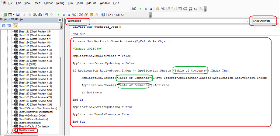
Assume you want the tab named "Table of Contents" to follow whenever you click on another tab . . .
Private Sub Workbook_SheetActivate(ByVal sh As Object)
'Update 20150306
Application.EnableEvents = False
Application.ScreenUpdating = False
If Application.ActiveSheet.Index <> Application.Sheets("Table of Contents").Index Then
Application.Sheets("Table of Contents").Move Before:=Application.Sheets(Application.ActiveSheet.Index)
Application.Sheets("Table of Contents").Activate
sh.Activate
End If
Application.ScreenUpdating = True
Application.EnableEvents = True
End Sub
Remove leading spaces in a cell | VBA (exceldome.com)
Sub Remove_leading_spaces_in_a_cell()
'declare a variable
Dim ws As Worksheet
Set ws = Worksheets("Analysis")
'Remove leading spaces in cell (B5)
ws.Range("C5") = LTrim(ws.Range("B5"))
End Sub
Renumber Duplicates in Column Headers
Option Explicit
Sub findDuplicatesDoSomethingPlease()
Dim ws As Worksheet
Set ws = ActiveWorkbook.Worksheets("dupeCols")
ws.Activate
Dim lastCol As Long
Dim thisCol As Long
Dim testCol As Long
Dim foundCount As Long
lastCol = ws.Cells(1, Columns.Count).End(xlToLeft).Column
For thisCol = 1 To lastCol - 1
If ws.Cells(1, thisCol).Value <> "" Then
foundCount = 0
For testCol = thisCol + 1 To lastCol
If Cells(1, thisCol).Value = Cells(1, testCol).Value Then
foundCount = foundCount + 1
Cells(1, testCol).Value = Cells(1, thisCol).Value & CStr(foundCount)
End If
Next testCol
End If
Next thisCol
End Sub
Renumber Duplicates in Rows 'use with Excel file here
Option Explicit
Sub findDuplicatesRowsDoSomethingPlease()
Dim ws As Worksheet
Set ws = ActiveWorkbook.Worksheets("dupeRows")
ws.Activate
Dim lastRow As Long
Dim thisRow As Long
Dim testRow As Long
Dim foundCount As Long
lastRow = ws.Range("A" & Rows.Count).End(xlUp).Row
'MsgBox "The # of rows is: " & lastRow
For thisRow = 1 To lastRow - 1
If ws.Cells(thisRow, 1).Value <> "" Then
foundCount = 0
For testRow = thisRow + 1 To lastRow
If Cells(thisRow, 1).Value = Cells(testRow, 1).Value Then
foundCount = foundCount + 1
Cells(testRow, 1).Value = Cells(thisRow, 1).Value & CStr(foundCount)
End If
Next testRow
End If
Next thisRow
End Sub
My video is here: https://youtu.be/ecqnexh-YCo
Option Explicit
Sub findAllBlankCellsInColumnA()
Dim shData, shOutput As Worksheet
Set shData = ThisWorkbook.Worksheets("Main")
Set shOutput = ThisWorkbook.Worksheets("output1")
Dim lr As Long
lr = Range("A" & Rows.Count).End(xlUp).Row
shData.Range("B1:B" & lr).SpecialCells(xlCellTypeBlanks).EntireRow.Copy shOutput.Range("A:K") 'here, Column B is what I'm using for blank cells search
End Sub
'source: https://stackoverflow.com/questions/25661659/select-all-blanks-cells-in-a-column
'Sheets("sheet1").Range("C:E").Copy Sheets("sheet2").Range("G:I")
Use a Workbook_Open event handler:
Sub Workbook_Open()
ActiveWorkbook.Sheets("OpenToThisSheet").Activate
End Sub
Again, change the sheet name to reflect the name of the actual sheet you want displayed. This event handler should be added as part of the ThisWorkbook module.
Source: Opening a Workbook to a Specific Worksheet (Microsoft Excel) (tips.net)
Here are some examples of date and time formats:
Sub date_and_time()
'Now => returns the current date and time (02.07.2012 09:09:02)
date_test = Now()
'Returns: 02.07.12
Range("A1") = Format(date_test, "mm.dd.yy")
'Returns: 7 February 2012
Range("A2") = Format(date_test, "d mmmm yyyy")
'Returns: February 7, 2012
Range("A3") = Format(date_test, "mmmm j, yyyy")
'Returns: Tue 07
Range("A4") = Format(date_test, "ddd dd")
'Returns: February-12
Range("A6") = Format(date_test, "mmmm-yy")
'Returns: 02.07.2012 09:09
Range("A7") = Format(date_test, "mm.dd.yyyy hh:mm")
'Returns: 2.7.12 9:09 AM
Range("A8") = Format(date_test, "m.d.yy h:mm AM/PM")
'Returns: 9H09
Range("A9") = Format(date_test, "h\Hmm")
End Sub
Source: VBA Tip: Display Formats for Date and Time (excel-pratique.com)
Dim a As Long
Dim b As Long
Dim c As Long
'Dim marks As String
Dim tally As Long
Dim numRows As Long
Dim lastrow As Long
Dim lastRow0 As Long
Dim lastRow1 As Long
Dim lastRow2 As Long
Dim n As Integer
Dim shData As Worksheet, shOutput As Worksheet
'Worksheets.Add.Name = "Expires60Days"
Set shData = ThisWorkbook.Worksheets("Main")
Set shOutput = ThisWorkbook.Worksheets("Expires60Days")
shOutput.Range("A1").CurrentRegion.Offset(1).Clear 'this clears BOTH content & formatting
'Get the range of "MergedColumnsFinal" worksheet
shData.Activate
Dim rg As Range
Set rg = shData.Range("A2").CurrentRegion 'this places you in A5 in 2020 tab & selects area with contiguous data
'The main code
Dim i, row As Long
row = 2 'you'll now start in row of the area that was selected as "CurrentRegion" . . .
For i = 2 To rg.Rows.Count
Dim dtToday As Date, marks As Variant
dtToday = Date
'MsgBox dtToday
marks = rg.Cells(i, 3).Value
'MsgBox marks
If marks <= dtToday + 60 Then
'Copy using selections
shOutput.Range("A" & row).Resize(1, rg.Columns.Count).Value = rg.Rows(i).Value
'move to the next output row
row = row + 1
End If
Next i
Worksheets("Expires60Days").Activate
Worksheets("Expires60Days").Range("A1:I1").Columns.AutoFit
With ActiveSheet
numRows = .Cells(.Rows.Count, "B").End(xlUp).row
.Range("K1").Value = numRows - 1
Range("A2", Range("I2").End(xlDown)).Sort Key1:=Range("C2"), Order1:=xlAscending, Header:=xlNo 'sort by column B2--after looking across from A2 to R2
End With
shOutput.Range("K2").Value = Format(Now(), "mm.dd.yyyy hh:mm")
End Sub
To populate an array based on text entries in an Excel worksheet using VBA, you can use the following steps:
Declare a variable to hold the array.
Dim myArray() As String
Determine the size of the array. You can do this by using the WorksheetFunction.CountA function to count the number of non-empty cells in a range. For example, if the text entries are in column A starting from row 1, you can use the following code to determine the size of the array:
Dim arraySize As Long arraySize = WorksheetFunction.CountA(Range("A:A"))
Re-dimension the array to the size determined in step 2.
ReDim myArray(1 To arraySize)
Loop through the range of cells containing the text entries and add each cell's value to the array.
For i = 1 To arraySize myArray(i) = Cells(i, 1).Value Next i
You can now use the array in your VBA code.
For example, you can loop through the array and perform some operation on each element:
For i = 1 To arraySize ' Perform some operation on myArray(i) Next i
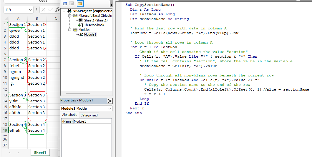
Sub CopySectionName()
Dim r As Long
Dim lastRow As Long
Dim sectionName As String
' Find the last row with data in column A
lastRow = Cells(Rows.Count, "A").End(xlUp).Row
' Loop through all rows in column A
For r = 1 To lastRow
' Check if the cell contains the value "section"
If Cells(r, "A").Value Like "*" & section & "*" Then
' If the cell contains "section", store the value in the variable
sectionName = Cells(r, "A").Value
' Loop through all non-blank rows beneath the current row
Do While r <= lastRow And Cells(r, "A").Value <> ""
' Copy the section name to the end of the row
Cells(r, Columns.Count).End(xlToLeft).Offset(0, 1).Value = sectionName
r = r + 1
Loop
End If
Next r
End Sub
Use with this Excel file
Use with this Excel sheet here
Sub PopulateValues()
Dim lastRow As Long, i As Long
Dim shData, shOutput As Worksheet
Set shData = ThisWorkbook.Worksheets("one")
Set shOutput = ThisWorkbook.Worksheets("two")
' Get the last row in Sheet2
lastRow = shOutput.Cells(shOutput.Rows.Count, "A").End(xlUp).Row
' Loop through each row in Sheet2
For i = 1 To lastRow
' Use VLOOKUP to check if the key in column A of Sheet2 exists in column A of Sheet1
Dim value As Variant
value = Application.WorksheetFunction.VLookup(shOutput.Cells(i, "A").value, shData.Range("A:B"), 2, False)
' If a match was found, write the associated value to column B of Sheet2
If Not IsError(value) Then
shOutput.Cells(i, "B").value = value
End If
Next i
End Sub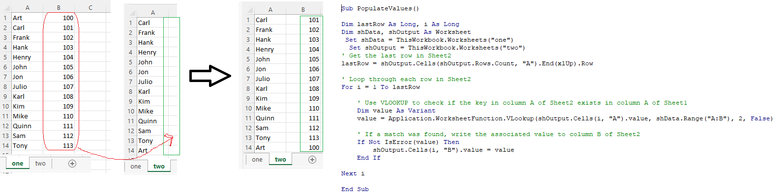
Filter by Column A and Column B, sort by column A and then column B
Sub GroupData()
Dim lastRow As Long
lastRow = ActiveSheet.Cells(ActiveSheet.Rows.Count, "A").End(xlUp).Row
With ActiveSheet
.Range("A1:C" & lastRow).AutoFilter Field:=1, Criteria1:="<>" ------can change to "A1:D" etc. if sheet has 4 columns of data, etc.
.Range("A1:C" & lastRow).AutoFilter Field:=2, Criteria1:="<>"
.Range("A2:C" & lastRow).Sort key1:=.Range("A2"), Order1:=xlAscending, Key2:=.Range("B2"), Order2:=xlAscending
.Range("A2:C" & lastRow).Group
End With
Columns.Sort key1:=Columns("A"), Order1:=xlAscending, Key2:=Columns("B"), Order2:=xlAscending, Header:=xlYes
End Sub
Use above code with this Excel file
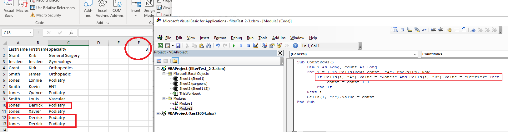
Count # of rows containing Certain Value in Column A and Column B and Enter Results into A Cell
Sub CountRows()
Dim i As Long, count As Long
For i = 1 To Cells(Rows.count, "A").End(xlUp).Row
If Cells(i, "A").Value = "Jones" And Cells(i, "B").Value = "Derrick" Then
count = count + 1
End If
Next i
Cells(1, "F").Value = count
End Sub
Sub CountRows()
Dim i As Long, count As Long
For i = 1 To Cells(Rows.count, "D").End(xlUp).Row
If Cells(i, "D").Value = "Jones" And Cells(i, "E").Value = "James" And Cells(i, "R").Value = "Not Met" Then
count = count + 1
End If
Next i
Cells(2, "AK").Value = count
End Sub
Sub CountRows()
Dim i As Long, count As Long
lastname = Range("AO1").Value 'here you enter the lastname you're seeking into cell AO1
firstname = Range("AP1").Value
For i = 1 To Cells(Rows.count, "D").End(xlUp).Row
If Cells(i, "D").Value = lastname And Cells(i, "E").Value = firstname Then
count = count + 1
End If
Next i
Cells(1, "AK").Value = count
End Sub
Sub CountRows()
Dim i As Long, count As Long
lastname = Range("AO1").Value
firstname = Range("AP1").Value
For i = 1 To Cells(Rows.count, "D").End(xlUp).Row
If Cells(i, "D").Value = lastname And Cells(i, "E").Value = firstname And Cells(i, "R").Value = "Not Met" Then
count = count + 1
End If
Next i
Cells(2, "AK").Value = count
End Sub
Sub CountRows()
Dim i As Long, count, count1 As Long
lastname = Range("AO1").Value
firstname = Range("AP1").Value
For i = 1 To Cells(Rows.count, "D").End(xlUp).Row
If Cells(i, "D").Value = lastname And Cells(i, "E").Value = firstname And Cells(i, "R").Value = "Not Met" Then
count = count + 1
End If
Next i
Cells(2, "AK").Value = count
For i = 1 To Cells(Rows.count, "D").End(xlUp).Row
If Cells(i, "D").Value = lastname And Cells(i, "E").Value = firstname And Cells(i, "T").Value = "Not Met" Then
count1 = count1 + 1
End If
Next i
Cells(3, "AK").Value = count1
End Sub
Use with this file here
Mother of all
Sub CountRows()
Dim i As Long, count, count1, count2, count3, count4, count5, count6, count7, count8, count9, count10, count11 As Long
lastname = Range("AO1").Value
firstname = Range("AP1").Value
For i = 1 To Cells(Rows.count, "D").End(xlUp).Row
If Cells(i, "D").Value = lastname And Cells(i, "E").Value = firstname And Cells(i, "R").Value = "Not Met" Then
count = count + 1
End If
Next i
Cells(2, "AK").Value = count
For i = 1 To Cells(Rows.count, "D").End(xlUp).Row
If Cells(i, "D").Value = lastname And Cells(i, "E").Value = firstname And Cells(i, "T").Value = "Not Met" Then
count1 = count1 + 1
End If
Next i
Cells(3, "AK").Value = count1
For i = 1 To Cells(Rows.count, "D").End(xlUp).Row
If Cells(i, "D").Value = lastname And Cells(i, "E").Value = firstname And Cells(i, "U").Value = "Not Met" Then
count2 = count2 + 1
End If
Next i
Cells(5, "AK").Value = count2
For i = 1 To Cells(Rows.count, "D").End(xlUp).Row
If Cells(i, "D").Value = lastname And Cells(i, "E").Value = firstname And Cells(i, "V").Value = "Not Met" Then
count3 = count3 + 1
End If
Next i
Cells(6, "AK").Value = count3
For i = 1 To Cells(Rows.count, "D").End(xlUp).Row
If Cells(i, "D").Value = lastname And Cells(i, "E").Value = firstname And Cells(i, "W").Value = "Not Met" Then
count4 = count4 + 1
End If
Next i
Cells(7, "AK").Value = count4
For i = 1 To Cells(Rows.count, "D").End(xlUp).Row
If Cells(i, "D").Value = lastname And Cells(i, "E").Value = firstname And Cells(i, "X").Value = "Not Met" Then
count5 = count5 + 1
End If
Next i
Cells(8, "AK").Value = count5
For i = 1 To Cells(Rows.count, "D").End(xlUp).Row
If Cells(i, "D").Value = lastname And Cells(i, "E").Value = firstname And Cells(i, "Y").Value = "Not Met" Then
count6 = count6 + 1
End If
Next i
Cells(9, "AK").Value = count6
For i = 1 To Cells(Rows.count, "D").End(xlUp).Row
If Cells(i, "D").Value = lastname And Cells(i, "E").Value = firstname And Cells(i, "Z").Value = "Not Met" Then
count7 = count7 + 1
End If
Next i
Cells(10, "AK").Value = count7
For i = 1 To Cells(Rows.count, "D").End(xlUp).Row
If Cells(i, "D").Value = lastname And Cells(i, "E").Value = firstname And Cells(i, "AA").Value = "Not Met" Then
count8 = count8 + 1
End If
Next i
Cells(11, "AK").Value = count8
For i = 1 To Cells(Rows.count, "D").End(xlUp).Row
If Cells(i, "D").Value = lastname And Cells(i, "E").Value = firstname And Cells(i, "AB").Value = "Not Met" Then
count9 = count9 + 1
End If
Next i
Cells(12, "AK").Value = count9
For i = 1 To Cells(Rows.count, "D").End(xlUp).Row
If Cells(i, "D").Value = lastname And Cells(i, "E").Value = firstname And Cells(i, "AC").Value = "Not Met" Then
count10 = count10 + 1
End If
Next i
Cells(13, "AK").Value = count10
For i = 1 To Cells(Rows.count, "D").End(xlUp).Row
If Cells(i, "D").Value = lastname And Cells(i, "E").Value = firstname And Cells(i, "AG").Value <> "Satisfactory" Then
count11 = count11 + 1
End If
Next i
Cells(14, "AK").Value = count11
End Sub
Use above with this file here
Sub CopyRows()
Dim sh1 As Worksheet, sh2 As Worksheet
Set sh1 = ThisWorkbook.Sheets("data")
Set sh2 = ThisWorkbook.Sheets("destiny")
'Get the values in cells AM1 and AN1 in Sheet2
Dim valueAM1 As String, valueAN1 As String
valueAM1 = sh2.Range("AM1").Value
valueAN1 = sh2.Range("AN1").Value
'Get the last row in Sheet1
Dim lastRow As Long
lastRow = sh1.Cells(sh1.Rows.Count, "A").End(xlUp).Row
'Iterate through each row in Sheet1
'enter lastname in AM1; enter a firstname in cell AN1 in sheet named destiny
For i = 2 To lastRow
'Check if the values in Column A and Column B match the values in Sheet2, Cells AM1 and AN1
If sh1.Cells(i, "D").Value = valueAM1 And sh1.Cells(i, "E").Value = valueAN1 Then
'Copy the row to Sheet2
sh1.Rows(i).Copy Destination:=sh2.Range("A" & sh2.Rows.Count).End(xlUp).Offset(1, 0)
End If
Next i
sh2.Rows(1).Value = sh1.Rows(1).Value
End Sub
Sub CountRowsWithValueInColumnR()
Dim lastRow As Long
Dim count As Long
Set sh2 = ThisWorkbook.Sheets("destiny")
Dim searchValue As Variant
searchValue = sh2.Range("AK1").Value
lastRow = sh2.Cells(sh2.Rows.count, "R").End(xlUp).Row
For i = 1 To lastRow
If sh2.Cells(i, "R").Value = searchValue Then
count = count + 1
End If
Next i
sh2.Range("AK2").Value = count
End Sub
Sub CountRowsWithValueInColumnR()
Dim lastRow As Long
Dim count, count1, count2, count3, count4, count5, count6, count7, count8, count9, count10, count11, count12 As Long
Set sh2 = ThisWorkbook.Sheets("destiny")
Dim searchValue As Variant
Dim lastnameProv, firstnameProv As String
lastnameProv = sh2.Range("D2").Value
firstnameProv = sh2.Range("E2").Value
sh2.Range("AK1").Value = "Not Met"
sh2.Range("AM1").Value = lastnameProv
sh2.Range("AN1").Value = firstnameProv
searchValue = sh2.Range("AK1").Value
lastRow = sh2.Cells(sh2.Rows.count, "R").End(xlUp).Row
For i = 1 To lastRow
If sh2.Cells(i, "R").Value = searchValue Then
count = count + 1
End If
Next i
If count = 0 Then
sh2.Range("AK2").Value = 0
Else
sh2.Range("AK2").Value = count
End If
For i = 1 To lastRow
If sh2.Cells(i, "S").Value = searchValue Then
count1 = count1 + 1
End If
Next i
If count1 = 0 Then
sh2.Range("AK3").Value = 0
Else
sh2.Range("AK3").Value = count1
End If
For i = 1 To lastRow
If sh2.Cells(i, "T").Value = searchValue Then
count2 = count2 + 1
End If
Next i
If count2 = 0 Then
sh2.Range("AK4").Value = 0
Else
sh2.Range("AK4").Value = count2
End If
For i = 1 To lastRow
If sh2.Cells(i, "U").Value = searchValue Then
count3 = count3 + 1
End If
Next i
If count3 = 0 Then
sh2.Range("AK5").Value = 0
Else
sh2.Range("AK5").Value = count3
End If
For i = 1 To lastRow
If sh2.Cells(i, "V").Value = searchValue Then
count4 = count4 + 1
End If
Next i
If count4 = 0 Then
sh2.Range("AK6").Value = 0
Else
sh2.Range("AK6").Value = count4
End If
For i = 1 To lastRow
If sh2.Cells(i, "W").Value = searchValue Then
count5 = count5 + 1
End If
Next i
If count5 = 0 Then
sh2.Range("AK7").Value = 0
Else
sh2.Range("AK7").Value = count5
End If
For i = 1 To lastRow
If sh2.Cells(i, "X").Value = searchValue Then
count6 = count6 + 1
End If
Next i
If count6 = 0 Then
sh2.Range("AK8").Value = 0
Else
sh2.Range("AK8").Value = count6
End If
For i = 1 To lastRow
If sh2.Cells(i, "Y").Value = searchValue Then
count7 = count7 + 1
End If
Next i
If count7 = 0 Then
sh2.Range("AK9").Value = 0
Else
sh2.Range("AK9").Value = count7
End If
For i = 1 To lastRow
If sh2.Cells(i, "Z").Value = searchValue Then
count8 = count8 + 1
End If
Next i
If count8 = 0 Then
sh2.Range("AK10").Value = 0
Else
sh2.Range("AK10").Value = count8
End If
For i = 1 To lastRow
If sh2.Cells(i, "AA").Value = searchValue Then
count9 = count9 + 1
End If
Next i
If count9 = 0 Then
sh2.Range("AK11").Value = 0
Else
sh2.Range("AK11").Value = count9
End If
For i = 1 To lastRow
If sh2.Cells(i, "AB").Value = searchValue Then
count10 = count10 + 1
End If
Next i
If count10 = 0 Then
sh2.Range("AK12").Value = 0
Else
sh2.Range("AK12").Value = count10
End If
For i = 1 To lastRow
If sh2.Cells(i, "AC").Value = searchValue Then
count11 = count11 + 1
End If
Next i
If count11 = 0 Then
sh2.Range("AK13").Value = 0
Else
sh2.Range("AK13").Value = count11
End If
End Sub
below is image for above code
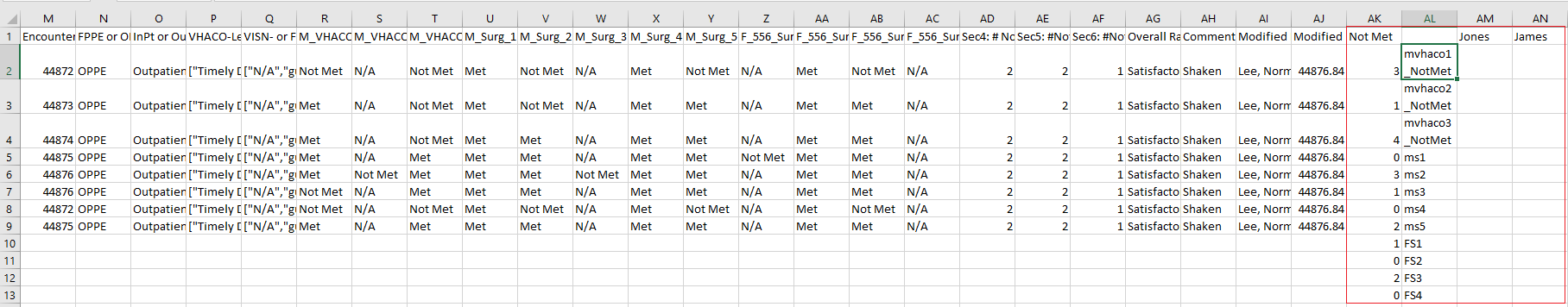
Sub CountRowsWithValueInColumnAB()
Dim lastRow As Long
Dim countA, count, count1, count2, count3, count4, count5, count6, count7, count8, count9, count10, count11, count12, count13 As Long
Set sh2 = ThisWorkbook.Sheets("data")
Set sh3 = ThisWorkbook.Sheets("form")
Dim searchValue As Variant
searchValue = "Not Met"
ratingValue = "Unsatisfactory"
lastRow = sh3.Cells(sh3.Rows.count, "AB").End(xlUp).Row
sh3.Range("C4").Value = lastRow - 1
For i = 1 To lastRow
If sh3.Cells(i, "AQ").Value = ratingValue Then
countA = countA + 1
End If
Next i
If countA = 0 Then
sh3.Range("G4").Value = 0
Else
sh3.Range("G4").Value = countA
End If
For i = 1 To lastRow
If sh3.Cells(i, "AB").Value = searchValue Then
count = count + 1
End If
Next i
If count = 0 Then
sh3.Range("C7").Value = 0
Else
sh3.Range("C7").Value = count
End If
For i = 1 To lastRow
If sh3.Cells(i, "AC").Value = searchValue Then
count1 = count1 + 1
End If
Next i
If count1 = 0 Then
sh3.Range("C8").Value = 0
Else
sh3.Range("C8").Value = count1
End If
For i = 1 To lastRow
If sh3.Cells(i, "AD").Value = searchValue Then
count2 = count2 + 1
End If
Next i
If count2 = 0 Then
sh3.Range("C9").Value = 0
Else
sh3.Range("C9").Value = count2
End If
For i = 1 To lastRow
If sh3.Cells(i, "AE").Value = searchValue Then
count3 = count3 + 1
End If
Next i
If count3 = 0 Then
sh3.Range("C10").Value = 0
Else
sh3.Range("C10").Value = count3
End If
For i = 1 To lastRow
If sh3.Cells(i, "AF").Value = searchValue Then
count4 = count4 + 1
End If
Next i
If count4 = 0 Then
sh3.Range("C11").Value = 0
Else
sh3.Range("C11").Value = count4
End If
For i = 1 To lastRow
If sh3.Cells(i, "AG").Value = searchValue Then
count5 = count5 + 1
End If
Next i
If count5 = 0 Then
sh3.Range("C12").Value = 0
Else
sh3.Range("C12").Value = count5
End If
For i = 1 To lastRow
If sh3.Cells(i, "AH").Value = searchValue Then
count6 = count6 + 1
End If
Next i
If count6 = 0 Then
sh3.Range("C13").Value = 0
Else
sh3.Range("C13").Value = count6
End If
For i = 1 To lastRow
If sh3.Cells(i, "AI").Value = searchValue Then
count7 = count7 + 1
End If
Next i
If count7 = 0 Then
sh3.Range("C14").Value = 0
Else
sh3.Range("C14").Value = count7
End If
For i = 1 To lastRow
If sh3.Cells(i, "AJ").Value = searchValue Then
count8 = count8 + 1
End If
Next i
If count8 = 0 Then
sh3.Range("C15").Value = 0
Else
sh3.Range("C15").Value = count8
End If
For i = 1 To lastRow
If sh3.Cells(i, "AK").Value = searchValue Then
count9 = count9 + 1
End If
Next i
If count9 = 0 Then
sh3.Range("C16").Value = 0
Else
sh3.Range("C16").Value = count9
End If
For i = 1 To lastRow
If sh3.Cells(i, "AL").Value = searchValue Then
count10 = count10 + 1
End If
Next i
If count10 = 0 Then
sh3.Range("C17").Value = 0
Else
sh3.Range("C17").Value = count10
End If
For i = 1 To lastRow
If sh3.Cells(i, "AM").Value = searchValue Then
count11 = count11 + 1
End If
Next i
If count11 = 0 Then
sh3.Range("C18").Value = 0
Else
sh3.Range("C18").Value = count11
End If
For i = 1 To lastRow
If sh3.Cells(i, "AN").Value = searchValue Then
count12 = count12 + 1
End If
Next i
If count11 = 0 Then
sh3.Range("C19").Value = 0
Else
sh3.Range("C19").Value = count12
End If
For i = 1 To lastRow
If sh3.Cells(i, "AO").Value = searchValue Then
count13 = count13 + 1
End If
Next i
If count11 = 0 Then
sh3.Range("C20").Value = 0
Else
sh3.Range("C20").Value = count13
End If
End Sub
*****Met below
Sub CountRowsWithMetValueInColumn()
Dim lastRow As Long
Dim countA, count, count1, count2, count3, count4, count5, count6, count7, count8, count9, count10, count11, count12, count13 As Long
Set sh2 = ThisWorkbook.Sheets("data")
Set sh3 = ThisWorkbook.Sheets("form")
Dim searchValue As Variant
searchValue = "Met"
lastRow = sh3.Cells(sh3.Rows.count, "AB").End(xlUp).Row
For i = 1 To lastRow
If sh3.Cells(i, "AB").Value = searchValue Then
count = count + 1
End If
Next i
If count = 0 Then
sh3.Range("E7").Value = 0
Else
sh3.Range("E7").Value = count
End If
For i = 1 To lastRow
If sh3.Cells(i, "AC").Value = searchValue Then
count1 = count1 + 1
End If
Next i
If count1 = 0 Then
sh3.Range("E8").Value = 0
Else
sh3.Range("E8").Value = count1
End If
For i = 1 To lastRow
If sh3.Cells(i, "AD").Value = searchValue Then
count2 = count2 + 1
End If
Next i
If count2 = 0 Then
sh3.Range("E9").Value = 0
Else
sh3.Range("E9").Value = count2
End If
For i = 1 To lastRow
If sh3.Cells(i, "AE").Value = searchValue Then
count3 = count3 + 1
End If
Next i
If count3 = 0 Then
sh3.Range("E10").Value = 0
Else
sh3.Range("E10").Value = count3
End If
For i = 1 To lastRow
If sh3.Cells(i, "AF").Value = searchValue Then
count4 = count4 + 1
End If
Next i
If count4 = 0 Then
sh3.Range("E11").Value = 0
Else
sh3.Range("E11").Value = count4
End If
For i = 1 To lastRow
If sh3.Cells(i, "AG").Value = searchValue Then
count5 = count5 + 1
End If
Next i
If count5 = 0 Then
sh3.Range("E12").Value = 0
Else
sh3.Range("E12").Value = count5
End If
For i = 1 To lastRow
If sh3.Cells(i, "AH").Value = searchValue Then
count6 = count6 + 1
End If
Next i
If count6 = 0 Then
sh3.Range("E13").Value = 0
Else
sh3.Range("E13").Value = count6
End If
For i = 1 To lastRow
If sh3.Cells(i, "AI").Value = searchValue Then
count7 = count7 + 1
End If
Next i
If count7 = 0 Then
sh3.Range("E14").Value = 0
Else
sh3.Range("E14").Value = count7
End If
For i = 1 To lastRow
If sh3.Cells(i, "AJ").Value = searchValue Then
count8 = count8 + 1
End If
Next i
If count8 = 0 Then
sh3.Range("E15").Value = 0
Else
sh3.Range("E15").Value = count8
End If
For i = 1 To lastRow
If sh3.Cells(i, "AK").Value = searchValue Then
count9 = count9 + 1
End If
Next i
If count9 = 0 Then
sh3.Range("E16").Value = 0
Else
sh3.Range("E16").Value = count9
End If
For i = 1 To lastRow
If sh3.Cells(i, "AL").Value = searchValue Then
count10 = count10 + 1
End If
Next i
If count10 = 0 Then
sh3.Range("E17").Value = 0
Else
sh3.Range("E17").Value = count10
End If
For i = 1 To lastRow
If sh3.Cells(i, "AM").Value = searchValue Then
count11 = count11 + 1
End If
Next i
If count11 = 0 Then
sh3.Range("E18").Value = 0
Else
sh3.Range("E18").Value = count11
End If
For i = 1 To lastRow
If sh3.Cells(i, "AN").Value = searchValue Then
count12 = count12 + 1
End If
Next i
If count11 = 0 Then
sh3.Range("E19").Value = 0
Else
sh3.Range("E19").Value = count12
End If
For i = 1 To lastRow
If sh3.Cells(i, "AO").Value = searchValue Then
count13 = count13 + 1
End If
Next i
If count11 = 0 Then
sh3.Range("E20").Value = 0
Else
sh3.Range("E20").Value = count13
End If
End Sub
*****N/A below
Sub CountRowsWithNAValueInColumn()
Dim lastRow As Long
Dim countA, count, count1, count2, count3, count4, count5, count6, count7, count8, count9, count10, count11, count12, count13 As Long
Set sh2 = ThisWorkbook.Sheets("data")
Set sh3 = ThisWorkbook.Sheets("form")
Dim searchValue As Variant
searchValue = "N/A"
lastRow = sh3.Cells(sh3.Rows.count, "AB").End(xlUp).Row
For i = 1 To lastRow
If sh3.Cells(i, "AB").Value = searchValue Then
count = count + 1
End If
Next i
If count = 0 Then
sh3.Range("F7").Value = 0
Else
sh3.Range("F7").Value = count
End If
For i = 1 To lastRow
If sh3.Cells(i, "AC").Value = searchValue Then
count1 = count1 + 1
End If
Next i
If count1 = 0 Then
sh3.Range("F8").Value = 0
Else
sh3.Range("F8").Value = count1
End If
For i = 1 To lastRow
If sh3.Cells(i, "AD").Value = searchValue Then
count2 = count2 + 1
End If
Next i
If count2 = 0 Then
sh3.Range("F9").Value = 0
Else
sh3.Range("F9").Value = count2
End If
For i = 1 To lastRow
If sh3.Cells(i, "AE").Value = searchValue Then
count3 = count3 + 1
End If
Next i
If count3 = 0 Then
sh3.Range("F10").Value = 0
Else
sh3.Range("F10").Value = count3
End If
For i = 1 To lastRow
If sh3.Cells(i, "AF").Value = searchValue Then
count4 = count4 + 1
End If
Next i
If count4 = 0 Then
sh3.Range("F11").Value = 0
Else
sh3.Range("F11").Value = count4
End If
For i = 1 To lastRow
If sh3.Cells(i, "AG").Value = searchValue Then
count5 = count5 + 1
End If
Next i
If count5 = 0 Then
sh3.Range("F12").Value = 0
Else
sh3.Range("F12").Value = count5
End If
For i = 1 To lastRow
If sh3.Cells(i, "AH").Value = searchValue Then
count6 = count6 + 1
End If
Next i
If count6 = 0 Then
sh3.Range("F13").Value = 0
Else
sh3.Range("F13").Value = count6
End If
For i = 1 To lastRow
If sh3.Cells(i, "AI").Value = searchValue Then
count7 = count7 + 1
End If
Next i
If count7 = 0 Then
sh3.Range("F14").Value = 0
Else
sh3.Range("F14").Value = count7
End If
For i = 1 To lastRow
If sh3.Cells(i, "AJ").Value = searchValue Then
count8 = count8 + 1
End If
Next i
If count8 = 0 Then
sh3.Range("F15").Value = 0
Else
sh3.Range("F15").Value = count8
End If
For i = 1 To lastRow
If sh3.Cells(i, "AK").Value = searchValue Then
count9 = count9 + 1
End If
Next i
If count9 = 0 Then
sh3.Range("F16").Value = 0
Else
sh3.Range("F16").Value = count9
End If
For i = 1 To lastRow
If sh3.Cells(i, "AL").Value = searchValue Then
count10 = count10 + 1
End If
Next i
If count10 = 0 Then
sh3.Range("F17").Value = 0
Else
sh3.Range("F17").Value = count10
End If
For i = 1 To lastRow
If sh3.Cells(i, "AM").Value = searchValue Then
count11 = count11 + 1
End If
Next i
If count11 = 0 Then
sh3.Range("F18").Value = 0
Else
sh3.Range("F18").Value = count11
End If
For i = 1 To lastRow
If sh3.Cells(i, "AN").Value = searchValue Then
count12 = count12 + 1
End If
Next i
If count11 = 0 Then
sh3.Range("F19").Value = 0
Else
sh3.Range("F19").Value = count12
End If
For i = 1 To lastRow
If sh3.Cells(i, "AO").Value = searchValue Then
count13 = count13 + 1
End If
Next i
If count11 = 0 Then
sh3.Range("F20").Value = 0
Else
sh3.Range("F20").Value = count13
End If
End Sub
use below with this Excel file here
Sub copyPasteOneSheet()
Dim providerLastname
Dim sh1 As Worksheet, sh2, sh3 As Worksheet
Set sh1 = ThisWorkbook.Sheets("data1")
'Get the values in cells AM1 and AN1 in data1
Dim valueAL1 As String, valueAM1 As String
valueAL1 = sh1.Range("AL2").Value
valueAM1 = sh1.Range("AM2").Value
'Get the last row in Sheet1
Dim lastRow As Long
lastRow = sh1.Cells(sh1.Rows.count, "A").End(xlUp).Row
sh1.Range("AL6:BU50").ClearContents
For i = 2 To lastRow
If sh1.Cells(i, "D").Value = valueAL1 And sh1.Cells(i, "E").Value = valueAM1 Then
Range(Cells(i, 1), Cells(i, 36)).Copy
Range("AL100").End(xlUp).Offset(1, 0).PasteSpecial xlPasteFormulasAndNumberFormats
End If
Next i
Range("AL2").Select
End Sub
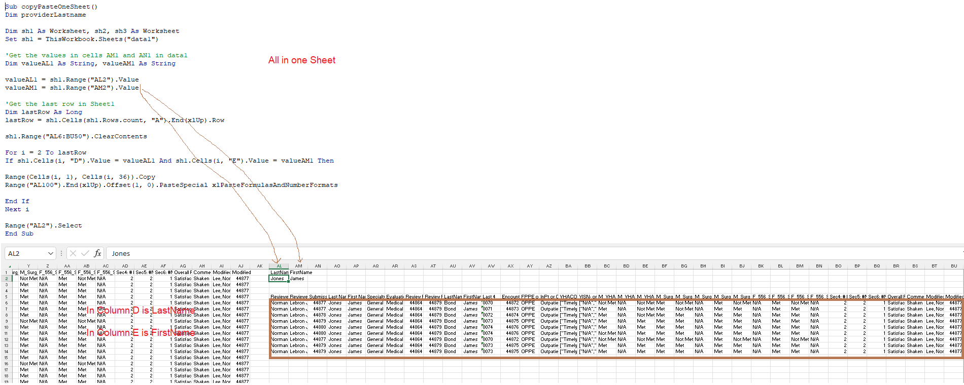
Source: EAF #37 - Excel VBA Loop to Find Records Matching Search Criteria - YouTube
This will copy row 1 and paste it into the existing row 5:
Range("1:1").Copy Range("5:5")
This will copy column C and paste it into column E:
Range("C:C").Copy Range("E:E")
' Set the string comparison method to Binary.

Option Compare Binary ' That is, "AAA" is less than "aaa".

' Set the string comparison method to Text.

Option Compare Text ' That is, "AAA" is equal to "aaa".
To protect a sheet in Excel but allow macros to run, you can follow these steps:
Open the Excel workbook containing the sheet you want to protect.
Click on the "Review" tab in the ribbon.
Click on "Protect Sheet" in the "Changes" group.
In the "Protect Sheet" dialog box, check the boxes next to the options you want to allow users to do on the protected sheet, such as "Select locked cells" and "Use AutoFilter." Make sure that the "Protect worksheet and contents of locked cells" box is checked.
Enter a password in the "Password to unprotect sheet" box, then click OK.
Open the Visual Basic Editor (VBE) by pressing "Alt + F11" on your keyboard.
In the VBE, select the sheet module of the sheet you just protected by clicking on it in the Project Explorer window.
In the module code, add the following line at the beginning of the code:
ActiveSheet.Unprotect Password:="yourpassword"
Add the following line at the end of the code:
ActiveSheet.Protect Password:="yourpassword"
Note: Replace "yourpassword" with the password you used to protect the sheet in step 5.
Save the workbook and close the VBE.
Now the sheet is protected and macros can still be run. When the macro runs, it will unprotect the sheet, perform the necessary actions, and then protect the sheet again.
Sub UnprotectAllSheets()
Dim ws As Worksheet
For Each ws In ActiveWorkbook.Worksheets
If ws.ProtectContents = True Then
ws.Unprotect Password:="yourpassword"
End If
Next ws
End Sub
Sub CopyDataWithFormattingAndColumnWidths()
Application.DisplayAlerts = False
'Copy data from Sheet1 to Sheet2 with formatting and column widths
Dim i As Integer
Dim j As Integer
. . . . .
destinationSheet.Range("A1").Select
Application.DisplayAlerts = True
End Sub
Source: VBA auto click ok on pop up box | MrExcel Message Board
Sub colorFont()
Dim lastRow As Long
Dim i, j As Long
Dim sh1 As Worksheet
Set sh1 = ThisWorkbook.Sheets("form")
lastRow = sh1.Cells(Rows.count, "AJ").End(xlUp).Row
For i = 1 To lastRow
If sh1.Range("AJ" & i).Value = "Unsatisfactory" Then
sh1.Range("AJ" & i).Font.Color = vbRed
End If
Next i
For i = 1 To lastRow
For j = 24 To 37
If sh1.Range(Cells(i, j), Cells(i, j)).Value = "Not Met" Then
sh1.Range(Cells(i, j), Cells(i, j)).Font.Color = vbRed
sh1.Range("P" & i).Font.Color = vbRed 'colors column P cell value red
End If
Next j
Next i
End Sub
Sub GetFileNamesInFolder()
Dim folderPath As String
Dim filesInFolder As Object
Dim file As Object
Dim i As Integer
' Specify the folder path
folderPath = "C:\YourFolderPath\" ' Change this to the path of your folder
' Clear existing data in column A
Columns("A:A").Clear
' Get the list of files in the folder
Set filesInFolder = CreateObject("Scripting.FileSystemObject").GetFolder(folderPath).Files
' Loop through each file and populate the column
i = 1
For Each file In filesInFolder
Cells(i, 1).Value = file.Name
i = i + 1
Next file
MsgBox "File names populated successfully!", vbInformation
End Sub
To save the PDFs directly in the folder where your Excel workbook is located:
ws.ExportAsFixedFormat Type:=xlTypePDF, Filename:=ThisWorkbook.Path & "\" & ws.Name & ".pdf", Quality:=xlQualityStandard
Sub PrintTabsStartingWithAppToPDF()
Dim ws As Worksheet
' Loop through each worksheet in the workbook
For Each ws In ThisWorkbook.Sheets
' Check if the sheet name starts with "App"
If Left(ws.Name, 3) = "App" Then
' Print the sheet to PDF
ws.ExportAsFixedFormat Type:=xlTypePDF, Filename:=ThisWorkbook.Path & "\" & ws.Name & ".pdf", Quality:=xlQualityStandard
End If
Next ws
End Sub
| Name | CO | DIV | Clinic | APPDATE | APPTTIME | Enter Date | Enter Clinic | ||
| Smith | 1 | 235 | REU | 7/14/2023 | 700 | 7/14/2023 | REU | ||
| Jones | 2 | 236 | XRAY | 8/1/2023 | 900 | ||||
| Lim | 3 | 237 | Eye | 1/2/2023 | 730 | ||||
| SmithC | 1 | 235 | REU | 11/2/2021 | 1000 | ||||
| June | 2 | 235 | REU | 7/14/2023 | 900 | ||||
Sub GenerateAppointmentWorksheets()
Dim wsSource As Worksheet
Dim nameCell As Range, wsNew As Worksheet
Dim statement As String
Dim lastRow As Long, i As Long
' Set the source worksheet
Set wsSource = ThisWorkbook.Sheets("Sheet1") ' Change the sheet name as needed
' Find the last row in column A
lastRow = wsSource.Cells(wsSource.Rows.Count, "A").End(xlUp).row
' Loop through each row in column "Name"
For i = 2 To lastRow ' Assuming data starts from row 2
' Get the name from the current row
Set nameCell = wsSource.Cells(i, 1)
' Create a new worksheet for each name
Set wsNew = Sheets.Add(After:=Sheets(Sheets.Count))
wsNew.Name = "Appointment_" & nameCell.Value
' Generate a statement for the appointment
statement = "You have an appointment with this clinic at this date and time."
' Customize the statement based on your data (e.g., add clinic name, date, time)
' For illustration, concatenate name, clinic, date, and time
statement = statement & vbCrLf & vbCrLf & "Name: " & nameCell.Value & vbCrLf & "Clinic: [ClinicName]" & vbCrLf & "Date: [AppointmentDate]"
' Replace placeholders with actual data
' Replace [ClinicName] and [AppointmentDate] with your actual column references
statement = Replace(statement, "[ClinicName]", wsSource.Cells(i, 4).Value) ' Assuming clinic name is in column D
statement = Replace(statement, "[AppointmentDate]", wsSource.Cells(i, 5).Value) ' Assuming appointment date is in column E
' Store the statement in the new worksheet
wsNew.Range("A1").Value = statement
Next i
End Sub
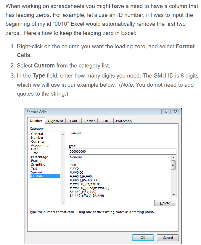
4 easy steps to keep the leading zero in Excel! (smu.edu)
How to hide the True/False words within cell when linked to checkbox in Excel? (extendoffice.com)
Word doc here
Sub CreateROSCheckbox()
Dim ws As Worksheet
Dim chkBox As checkBox
' Set the worksheet
Set ws = ThisWorkbook.Sheets("Sheet3") ' Replace "Sheet1" with your sheet name
' Define the position for the checkbox
Dim leftPos As Single
Dim topPos As Single
Dim widthSize As Single
Dim heightSize As Single
leftPos = 10
topPos = 10
widthSize = 100
heightSize = 15
' Create the checkbox
Set chkBox = ws.CheckBoxes.Add(leftPos, topPos, widthSize, heightSize)
' Set checkbox properties
With chkBox
.Name = "CheckBoxROS"
.Caption = "ROS"
.LinkedCell = ws.Range("A1").Address ' Replace A1 with the cell you want to link
End With
End Sub
If UCase(.Cells(r, 11).Value) = UCase(Environ("Username")) Then
VBA: How to find a match that NOT Case-sensitive? | MrExcel Message Board
Dim wsSource, wsOutput, wsLetter, wsActions As Worksheet
Dim lastRow, i, row As Long
' Set references to worksheets
Set wsSource = ThisWorkbook.Sheets("Main")
Set wsOutput = ThisWorkbook.Sheets("Output")
Set wsActions = ThisWorkbook.Sheets("Actions")
' Clear existing data in Sheet2
wsOutput.UsedRange.Clear
' Find the last row in Sheet1
lastRow = wsSource.Cells(wsSource.Rows.
Dim PtName As String 'Declare PtName as a String variable
CommentsAll = wsActions.Range("B10").Value
Dim rg As Range
Set rg = wsSource.Range("A2").
'The main code
row = 2
For i = 2 To rg.Rows.Count 'Assuming data starts from row 2
'Loop through each row in Sheet1 and filter based on conditions
'If UCase(.Cells(r, 11).Value) = UCase(Environ("Username")) Then
'If rg.Cells(i, 1).Value Like "*" & PtName & "*" Then
'if you need to find a word in either column H or I, use this below:
'If UCase(rg.Cells(i, 8).Value) Like UCase("*" & CommentsAll & "*") Or UCase(rg.Cells(i, 9).Value) Like UCase("*" & CommentsAll & "*") Then
If UCase(rg.Cells(i, 8).Value) Like UCase("*" & CommentsAll & "*") Then
wsOutput.Range("A" & row).Resize(1, rg.Columns.Count).Value = rg.Rows(i).Value
'move to the next output row
row = row + 1
End If
Next i
wsSource.Rows(1).Copy Destination:=wsOutput.Rows(1)
wsOutput.Columns("G:G").
Application.CutCopyMode = False
wsOutput.Activate
MsgBox "Here are the results of filtering using Comments", vbInformation, "Filter Information"
End Sub
Sub UnhideMe() 'Unhide all of the sheets which are hidden in an Excel file.
Dim ws As Worksheet
For Each ws In Sheets
ws.Visible=True
Next ws
End Sub

Code for "btnSubmitLast4" Submit button is below:
Private Sub btnSubmitLast4_Click()
Dim a As String
a = Me.tboxLast4a.Value
Dim i, LastRow
Dim LastRow1 As Long
LastRow = Sheets("Aggregate").Range("A" & Rows.Count).End(xlUp).row
Sheets("SelProv").Range("A2:I100").ClearContents
For i = 2 To LastRow
If Sheets("Aggregate").Cells(i, "B").Value = a Then
Sheets("Aggregate").Cells(i, "B").EntireRow.Copy Destination:=Sheets("SelProv").Range("A" & Rows.Count).End(xlUp).Offset(1)
End If
Next i
LastRow1 = ThisWorkbook.Sheets("SelProv").Cells(Rows.Count, 1).End(xlUp).Offset(-1).row
MsgBox ThisWorkbook.Sheets("SelProv").Range("A2").Value & " has " & LastRow1 & " intubations recorded in this database", vbOKCancel
LastRow1 = 0
End Sub
Sub UnhideMe() 'Unhide all of the sheets which are hidden in an Excel file.
Dim ws As Worksheet
For Each ws In Sheets
ws.Visible=True
Next ws
End Sub
Sub ListAndConcatenateFiles()
Dim ws As Worksheet
Dim folderPath As String
Dim fileName As String
Dim filePath As String
Dim rowNum As Long
' Specify the worksheet where you want to list the files
Set ws = ThisWorkbook.Sheets("Sheet1")
' Specify the folder path
folderPath = "C:\Users\norml\OneDrive\Pictures\pulm_GE\pulm_TMP\" ' Update with the actual folder path
' Check if the folder exists
If Dir(folderPath, vbDirectory) = "" Then
MsgBox "Folder not found.", vbExclamation
Exit Sub
End If
' Clear existing data in column C
ws.Range("C:C").ClearContents
' Initialize row number
rowNum = 2
' Loop through each file in the folder
fileName = Dir(folderPath & "\*.*")
Do While fileName <> ""
' Check if the item is a file (not a folder)
If Not (GetAttr(folderPath & "\" & fileName) And vbDirectory) = vbDirectory Then
' Concatenate file path with URL
filePath = "http://www.medical-life-skills.com/medschool/pulm/pulm_TMP/" & fileName
' Place concatenated URL in column C
ws.Cells(rowNum, "C").Value = filePath
' Move to the next row
rowNum = rowNum + 1
End If
' Get the next file name
fileName = Dir
Loop
' Display a message box indicating the files are listed and concatenated
MsgBox "Files listed and concatenated successfully!", vbInformation
End Sub
Sub SendEmailsWithTable()
Dim OutApp As Object
Dim OutMail As Object
Dim ws As Worksheet
Dim lastRow As Long
Dim i As Long
Dim emailAddr As String
Dim headerRange As Range
Dim dataRange As Range
Dim emailBody As String
' Set the worksheet
Set ws = ThisWorkbook.Sheets("Sheet1") ' Update "Sheet1" with your sheet name
' Find the last row with data in Column C
lastRow = ws.Cells(ws.Rows.Count, "C").End(xlUp).Row
' Loop through each row in the worksheet
For i = 2 To lastRow ' Assuming headers are in row 1, start from row 2
' Check if email address is not empty
If ws.Cells(i, "C").Value <> "" Then
' Get the email address
emailAddr = ws.Cells(i, "C").Value
' Create the email body with a table
emailBody = "<html><body><table border='1' cellpadding='5' cellspacing='0'><tr>"
' Copy headers from Sheet1
Set headerRange = ws.Range("A1", ws.Cells(1, ws.Columns.Count).End(xlToLeft))
For Each cell In headerRange
emailBody = emailBody & "<th>" & cell.Value & "</th>" ' Create table header
Next cell
emailBody = emailBody & "</tr>"
' Copy the corresponding row data to the email body table
Set dataRange = ws.Range("A" & i, ws.Cells(i, ws.Columns.Count).End(xlToLeft))
emailBody = emailBody & "<tr>"
For Each cell In dataRange
emailBody = emailBody & "<td>" & cell.Value & "</td>" ' Create table data
Next cell
emailBody = emailBody & "</tr></table></body></html>
Sub SendEmailsWithAlerts()
Dim OutApp As Object
Dim OutMail As Object
Dim ws As Worksheet
Dim lastRow As Long
Dim i As Long
Dim emailAddr As String
Dim headerRange As Range
Dim dataRange As Range
Dim emailBody As String
' Set the worksheet
Set ws = ThisWorkbook.Sheets("Sheet1") ' Update "Sheet1" with your sheet name
' Find the last row with data in Column C
lastRow = ws.Cells(ws.Rows.Count, "C").End(xlUp).Row
' Loop through each row in the worksheet
For i = 2 To lastRow ' Assuming headers are in row 1, start from row 2
' Check if email address is not empty
If ws.Cells(i, "C").Value <> "" Then
' Get the email address
emailAddr = ws.Cells(i, "C").Value
' Create the email subject
Dim subjectLine As String
subjectLine = "You have alerts in CPRS to clear: please log in to CPRS read-only to clear especially the CRITICAL & Abnormal ones"
' Create the email body with a table
emailBody = "<html><body><h2>" & subjectLine & "</h2><table border='1' cellpadding='5' cellspacing='0'><tr style='font-weight:bold;'>"
' Copy headers from Sheet1
Set headerRange = ws.Range("A1", ws.Cells(1, ws.Columns.Count).End(xlToLeft))
For Each cell In headerRange
emailBody = emailBody & "<th>" & cell.Value & "</th>" ' Create table header
Next cell
emailBody = emailBody & "</tr>"
' Copy the corresponding row data to the email body table
Set dataRange = ws.Range("A" & i, ws.Cells(i, ws.Columns.Count).End(xlToLeft))
emailBody = emailBody & "<tr>"
For Each cell In dataRange
emailBody = emailBody & "<td>" & cell.Value & "</td>" ' Create table data
Next cell
emailBody = emailBody & "</tr></table></body></html>